

16.3 Elastic–Plastic Inflation of a Spherical Vessel
229
where
q 0 = q
c 3
b 3 − c 3 .
For the plastic zone, let us use the solution (16.31) in the boundary
conditions
r = a : σ r = −p; r = c : σ r = −q.
(16.37)
We obtain
−p = 2σ s ln a + C 1 ,
−q = 2σ s ln c + C 1 .
(16.38)
Equations (16.38) contain three unknown values: C 1 , q, and c. To find
them, we must make another equation. The condition of displacement
continuity u at the boundary of the elastic and plastic zones can be used.
However, the condition σ ϕ − σ r = σ s at r → c + 0 is more convenient.
Indeed,
(σ ϕ − σ r )
r=c+0
= q 0
1 −
b 3
c 3 − 1 +
b 3
c 3
= σ s ,
for example,
3
2
q 0
b 3
c 3 = σ s .
(16.39)
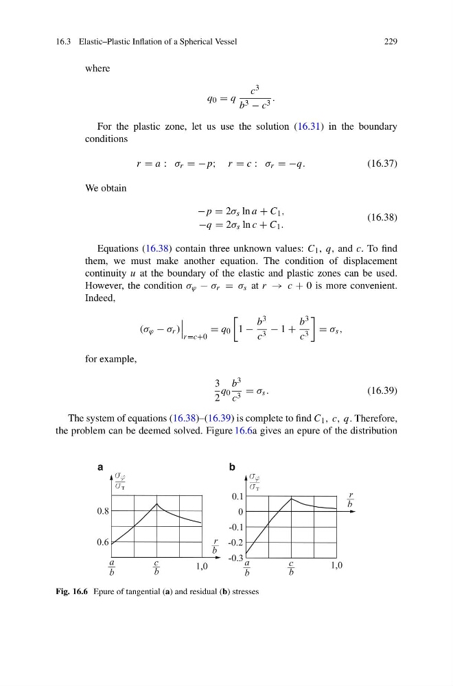
The system of equations (16.38)–(16.39) is complete to find C 1 , c, q. Therefore,
the problem can be deemed solved. Figure 16.6a gives an epure of the distribution
a
b
Fig. 16.6 Epure of tangential (a) and residual (b) stresses
229
where
q 0 = q
c 3
b 3 − c 3 .
For the plastic zone, let us use the solution (16.31) in the boundary
conditions
r = a : σ r = −p; r = c : σ r = −q.
(16.37)
We obtain
−p = 2σ s ln a + C 1 ,
−q = 2σ s ln c + C 1 .
(16.38)
Equations (16.38) contain three unknown values: C 1 , q, and c. To find
them, we must make another equation. The condition of displacement
continuity u at the boundary of the elastic and plastic zones can be used.
However, the condition σ ϕ − σ r = σ s at r → c + 0 is more convenient.
Indeed,
(σ ϕ − σ r )
r=c+0
= q 0
1 −
b 3
c 3 − 1 +
b 3
c 3
= σ s ,
for example,
3
2
q 0
b 3
c 3 = σ s .
(16.39)
The system of equations (16.38)–(16.39) is complete to find C 1 , c, q. Therefore,
the problem can be deemed solved. Figure 16.6a gives an epure of the distribution
a
b
Fig. 16.6 Epure of tangential (a) and residual (b) stresses