

11.12 Stability Under Non-conservative Load (Example)
139
The question arises: how significant can this difference be?
Obviously, the inequality (11.50) goes to (11.49) when f =
1
4ρ 2 . As already
noted, this value is the maximum and is reached when
b 2 = b 1 ρ
2 .
(11.51)
The expressions (11.37) and (11.38) show that the left side of the inequality
(11.50) depends on the parameters γ, μ, a and η. Denote the smallest positive
values of the parameter γ , for which the condition (11.50) is violated, by γ 0
μ (a, η),
and those of them that correspond to R max will be denoted by γ 0
∗ (a, η).
Since the function f (μ) is positive, it is obvious that at the given parameters a
and η, the value of γ 0
∗ (a, η) exceeds, as a rule, the corresponding value of γ 0
μ (a, η).
Therefore, at b 2 = b 1 ρ 2 , or at μ =
1
ρ 2 , the stability loss usually occurs later than at
other values of μ. Therefore, if the coefficients of small friction satisfy the relation
(11.51), then friction will be called b e s t.
The minimum values of γ 0
μ (a, η), as previously defined, are γ ∗ (η) and are
reached at f = 0 when μ → 0 or μ → ∞. In this case, friction is calledw o r s t.
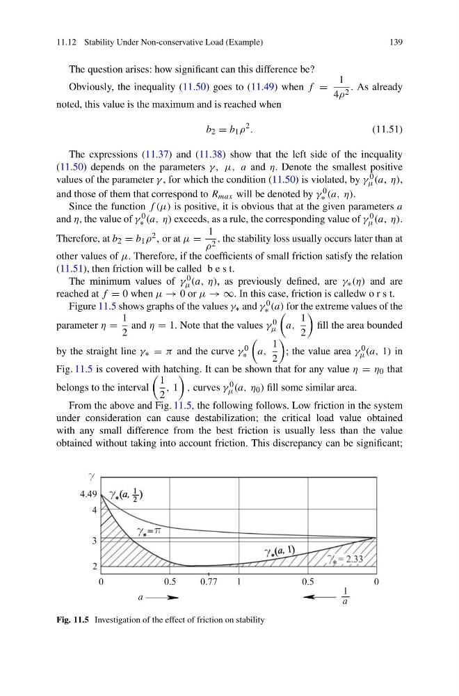
Figure 11.5 shows graphs of the values γ ∗ and γ 0
∗ (a) for the extreme values of the
parameter η =
1
2
and η = 1. Note that the values γ 0
μ
a,
1
2
fill the area bounded
by the straight line γ ∗ = π and the curve γ 0
∗
a,
1
2
; the value area γ 0
μ (a, 1) in
Fig. 11.5 is covered with hatching. It can be shown that for any value η = η 0 that
belongs to the interval
1
2
, 1
, curves γ 0
μ (a, η 0 ) fill some similar area.
From the above and Fig. 11.5, the following follows. Low friction in the system
under consideration can cause destabilization; the critical load value obtained
with any small difference from the best friction is usually less than the value
obtained without taking into account friction. This discrepancy can be significant;
Fig. 11.5 Investigation of the effect of friction on stability
139
The question arises: how significant can this difference be?
Obviously, the inequality (11.50) goes to (11.49) when f =
1
4ρ 2 . As already
noted, this value is the maximum and is reached when
b 2 = b 1 ρ
2 .
(11.51)
The expressions (11.37) and (11.38) show that the left side of the inequality
(11.50) depends on the parameters γ, μ, a and η. Denote the smallest positive
values of the parameter γ , for which the condition (11.50) is violated, by γ 0
μ (a, η),
and those of them that correspond to R max will be denoted by γ 0
∗ (a, η).
Since the function f (μ) is positive, it is obvious that at the given parameters a
and η, the value of γ 0
∗ (a, η) exceeds, as a rule, the corresponding value of γ 0
μ (a, η).
Therefore, at b 2 = b 1 ρ 2 , or at μ =
1
ρ 2 , the stability loss usually occurs later than at
other values of μ. Therefore, if the coefficients of small friction satisfy the relation
(11.51), then friction will be called b e s t.
The minimum values of γ 0
μ (a, η), as previously defined, are γ ∗ (η) and are
reached at f = 0 when μ → 0 or μ → ∞. In this case, friction is calledw o r s t.
Figure 11.5 shows graphs of the values γ ∗ and γ 0
∗ (a) for the extreme values of the
parameter η =
1
2
and η = 1. Note that the values γ 0
μ
a,
1
2
fill the area bounded
by the straight line γ ∗ = π and the curve γ 0
∗
a,
1
2
; the value area γ 0
μ (a, 1) in
Fig. 11.5 is covered with hatching. It can be shown that for any value η = η 0 that
belongs to the interval
1
2
, 1
, curves γ 0
μ (a, η 0 ) fill some similar area.
From the above and Fig. 11.5, the following follows. Low friction in the system
under consideration can cause destabilization; the critical load value obtained
with any small difference from the best friction is usually less than the value
obtained without taking into account friction. This discrepancy can be significant;
Fig. 11.5 Investigation of the effect of friction on stability