

5 Numerical Simulation of Taylor Vortex Flows …
55
the radius is 0 at that time. Then instability develops, which leads to the formation
of motion in all directions. The interesting fact is that the solution is reconstructed
in a catastrophic manner, i.e., the given character of the flow is preserved over a
certain time interval, then the surge of motion in the radial direction and along the
axis of the cylinders occurs, and it is relatively small compared to the motion in the
circumferential direction, but the solution changes qualitatively in the end. The flow
in this case becomes three-dimensional. Then, upon reaching the stationary solution,
the axisymmetric nature of the flow is established. When calculating with a change
in the L parameter, the same solution is obtained; the process of establishing it is not
accompanied by significant restructuring of the nature of the flow.
Figure 5.4c, d demonstrates an example of the restructuring of the flow at L
= 1.393 in an analogous form. In this case, when calculating with an increase of
parameter L, the nature of the flow with one pair of the vortices is determined by the
initial field of the flow, and this flow character is preserved. When calculating for the
flow with a discontinuity, two pairs of the Taylor vortices are formed. In fact, two
different solutions are possible at one L value.
Figure 5.4e, f demonstrates an example of the restructuring of the flow at L =
1.578 in a similar form. In this case, when calculating with an increase of parameter
L, the flow with one pair of the vortices re-forms into the flow with two pairs of the
vortices. When calculating for the flow with a discontinuity, two pairs of the Taylor
vortices are formed. The solutions are the same.
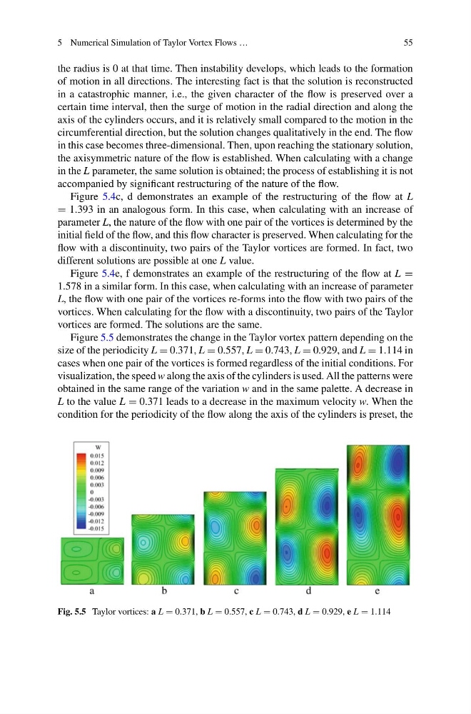
Figure 5.5 demonstrates the change in the Taylor vortex pattern depending on the
size of the periodicity L = 0.371, L = 0.557, L = 0.743, L = 0.929, and L = 1.114 in
cases when one pair of the vortices is formed regardless of the initial conditions. For
visualization, the speed w along the axis of the cylinders is used. All the patterns were
obtained in the same range of the variation w and in the same palette. A decrease in
L to the value L = 0.371 leads to a decrease in the maximum velocity w. When the
condition for the periodicity of the flow along the axis of the cylinders is preset, the
Fig. 5.5 Taylor vortices: a L = 0.371, b L = 0.557, c L = 0.743, d L = 0.929, e L = 1.114
55
the radius is 0 at that time. Then instability develops, which leads to the formation
of motion in all directions. The interesting fact is that the solution is reconstructed
in a catastrophic manner, i.e., the given character of the flow is preserved over a
certain time interval, then the surge of motion in the radial direction and along the
axis of the cylinders occurs, and it is relatively small compared to the motion in the
circumferential direction, but the solution changes qualitatively in the end. The flow
in this case becomes three-dimensional. Then, upon reaching the stationary solution,
the axisymmetric nature of the flow is established. When calculating with a change
in the L parameter, the same solution is obtained; the process of establishing it is not
accompanied by significant restructuring of the nature of the flow.
Figure 5.4c, d demonstrates an example of the restructuring of the flow at L
= 1.393 in an analogous form. In this case, when calculating with an increase of
parameter L, the nature of the flow with one pair of the vortices is determined by the
initial field of the flow, and this flow character is preserved. When calculating for the
flow with a discontinuity, two pairs of the Taylor vortices are formed. In fact, two
different solutions are possible at one L value.
Figure 5.4e, f demonstrates an example of the restructuring of the flow at L =
1.578 in a similar form. In this case, when calculating with an increase of parameter
L, the flow with one pair of the vortices re-forms into the flow with two pairs of the
vortices. When calculating for the flow with a discontinuity, two pairs of the Taylor
vortices are formed. The solutions are the same.
Figure 5.5 demonstrates the change in the Taylor vortex pattern depending on the
size of the periodicity L = 0.371, L = 0.557, L = 0.743, L = 0.929, and L = 1.114 in
cases when one pair of the vortices is formed regardless of the initial conditions. For
visualization, the speed w along the axis of the cylinders is used. All the patterns were
obtained in the same range of the variation w and in the same palette. A decrease in
L to the value L = 0.371 leads to a decrease in the maximum velocity w. When the
condition for the periodicity of the flow along the axis of the cylinders is preset, the
Fig. 5.5 Taylor vortices: a L = 0.371, b L = 0.557, c L = 0.743, d L = 0.929, e L = 1.114