

5 Numerical Simulation of Taylor Vortex Flows …
53
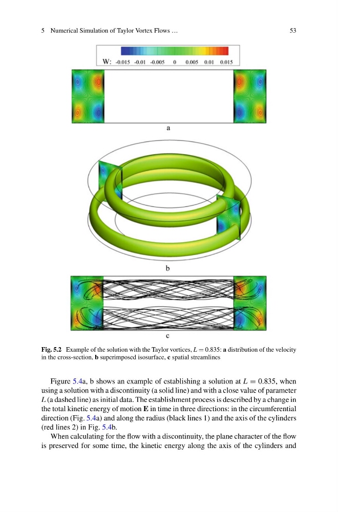
Fig. 5.2 Example of the solution with the Taylor vortices, L = 0.835: a distribution of the velocity
in the cross-section, b superimposed isosurface, c spatial streamlines
Figure 5.4a, b shows an example of establishing a solution at L = 0.835, when
using a solution with a discontinuity (a solid line) and with a close value of parameter
L (a dashed line) as initial data. The establishment process is described by a change in
the total kinetic energy of motion E in time in three directions: in the circumferential
direction (Fig. 5.4a) and along the radius (black lines 1) and the axis of the cylinders
(red lines 2) in Fig. 5.4b.
When calculating for the flow with a discontinuity, the plane character of the flow
is preserved for some time, the kinetic energy along the axis of the cylinders and
53
Fig. 5.2 Example of the solution with the Taylor vortices, L = 0.835: a distribution of the velocity
in the cross-section, b superimposed isosurface, c spatial streamlines
Figure 5.4a, b shows an example of establishing a solution at L = 0.835, when
using a solution with a discontinuity (a solid line) and with a close value of parameter
L (a dashed line) as initial data. The establishment process is described by a change in
the total kinetic energy of motion E in time in three directions: in the circumferential
direction (Fig. 5.4a) and along the radius (black lines 1) and the axis of the cylinders
(red lines 2) in Fig. 5.4b.
When calculating for the flow with a discontinuity, the plane character of the flow
is preserved for some time, the kinetic energy along the axis of the cylinders and