

50
F. A. Maksimov
move to the arbitrary curvilinear coordinate system. We will set the uniform grid
for the difference approximation of the initial equations in the following coordinate
system:
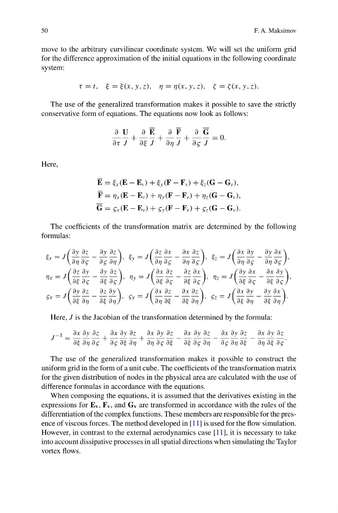
τ = t, ξ = ξ(x, y, z), η = η(x, y, z), ζ = ζ(x, y, z).
The use of the generalized transformation makes it possible to save the strictly
conservative form of equations. The equations now look as follows:
∂
∂τ
U
J
+
∂
∂ξ
E
J
+
∂
∂η
F
J
+
∂
∂ς
G
J
= 0.
Here,
E = ξ x (E − E v ) + ξ y (F − F v ) + ξ z (G − G v ),
F = η x (E − E v ) + η y (F − F v ) + η z (G − G v ),
G = ς x (E − E v ) + ς y (F − F v ) + ς z (G − G v ).
The coefficients of the transformation matrix are determined by the following
formulas:
ξ x = J
∂ y
∂η
∂z
∂ς
−
∂ y
∂ς
∂z
∂η
, ξ y = J
∂z
∂η
∂ x
∂ς
−
∂ x
∂η
∂z
∂ς
, ξ z = J
∂ x
∂η
∂ y
∂ς
−
∂ y
∂η
∂ x
∂ς
,
η x = J
∂z
∂ξ
∂ y
∂ς
−
∂ y
∂ξ
∂z
∂ς
, η y = J
∂ x
∂ξ
∂z
∂ς
−
∂z
∂ξ
∂ x
∂ς
, η z = J
∂ y
∂ξ
∂ x
∂ς
−
∂ x
∂ξ
∂ y
∂ς
,
ς x = J
∂ y
∂ξ
∂z
∂η
−
∂z
∂ξ
∂ y
∂η
, ς y = J
∂ x
∂η
∂z
∂ξ
−
∂ x
∂ξ
∂z
∂η
, ς z = J
∂ x
∂ξ
∂ y
∂η
−
∂ y
∂ξ
∂ x
∂η
.
Here, J is the Jacobian of the transformation determined by the formula:
J −1 =
∂ x
∂ξ
∂ y
∂η
∂z
∂ς
+
∂ x
∂ς
∂ y
∂ξ
∂z
∂η
+
∂ x
∂η
∂ y
∂ς
∂z
∂ξ
−
∂ x
∂ξ
∂ y
∂ς
∂z
∂η
−
∂ x
∂ς
∂ y
∂η
∂z
∂ξ
−
∂ x
∂η
∂ y
∂ξ
∂z
∂ς
.
The use of the generalized transformation makes it possible to construct the
uniform grid in the form of a unit cube. The coefficients of the transformation matrix
for the given distribution of nodes in the physical area are calculated with the use of
difference formulas in accordance with the equations.
When composing the equations, it is assumed that the derivatives existing in the
expressions for E v , F v , and G v are transformed in accordance with the rules of the
differentiation of the complex functions. These members are responsible for the presence of viscous forces. The method developed in [11] is used for the flow simulation.
However, in contrast to the external aerodynamics case [11], it is necessary to take
into account dissipative processes in all spatial directions when simulating the Taylor
vortex flows.
F. A. Maksimov
move to the arbitrary curvilinear coordinate system. We will set the uniform grid
for the difference approximation of the initial equations in the following coordinate
system:
τ = t, ξ = ξ(x, y, z), η = η(x, y, z), ζ = ζ(x, y, z).
The use of the generalized transformation makes it possible to save the strictly
conservative form of equations. The equations now look as follows:
∂
∂τ
U
J
+
∂
∂ξ
E
J
+
∂
∂η
F
J
+
∂
∂ς
G
J
= 0.
Here,
E = ξ x (E − E v ) + ξ y (F − F v ) + ξ z (G − G v ),
F = η x (E − E v ) + η y (F − F v ) + η z (G − G v ),
G = ς x (E − E v ) + ς y (F − F v ) + ς z (G − G v ).
The coefficients of the transformation matrix are determined by the following
formulas:
ξ x = J
∂ y
∂η
∂z
∂ς
−
∂ y
∂ς
∂z
∂η
, ξ y = J
∂z
∂η
∂ x
∂ς
−
∂ x
∂η
∂z
∂ς
, ξ z = J
∂ x
∂η
∂ y
∂ς
−
∂ y
∂η
∂ x
∂ς
,
η x = J
∂z
∂ξ
∂ y
∂ς
−
∂ y
∂ξ
∂z
∂ς
, η y = J
∂ x
∂ξ
∂z
∂ς
−
∂z
∂ξ
∂ x
∂ς
, η z = J
∂ y
∂ξ
∂ x
∂ς
−
∂ x
∂ξ
∂ y
∂ς
,
ς x = J
∂ y
∂ξ
∂z
∂η
−
∂z
∂ξ
∂ y
∂η
, ς y = J
∂ x
∂η
∂z
∂ξ
−
∂ x
∂ξ
∂z
∂η
, ς z = J
∂ x
∂ξ
∂ y
∂η
−
∂ y
∂ξ
∂ x
∂η
.
Here, J is the Jacobian of the transformation determined by the formula:
J −1 =
∂ x
∂ξ
∂ y
∂η
∂z
∂ς
+
∂ x
∂ς
∂ y
∂ξ
∂z
∂η
+
∂ x
∂η
∂ y
∂ς
∂z
∂ξ
−
∂ x
∂ξ
∂ y
∂ς
∂z
∂η
−
∂ x
∂ς
∂ y
∂η
∂z
∂ξ
−
∂ x
∂η
∂ y
∂ξ
∂z
∂ς
.
The use of the generalized transformation makes it possible to construct the
uniform grid in the form of a unit cube. The coefficients of the transformation matrix
for the given distribution of nodes in the physical area are calculated with the use of
difference formulas in accordance with the equations.
When composing the equations, it is assumed that the derivatives existing in the
expressions for E v , F v , and G v are transformed in accordance with the rules of the
differentiation of the complex functions. These members are responsible for the presence of viscous forces. The method developed in [11] is used for the flow simulation.
However, in contrast to the external aerodynamics case [11], it is necessary to take
into account dissipative processes in all spatial directions when simulating the Taylor
vortex flows.