

48
F. A. Maksimov
the implemented solution depends on different factors such as the mode of reaching
the stationary solution, the geometric peculiarities that enable the formation of the
vortices with the assigned size, and so on.
A large number of studies of the Taylor vortex flow have been performed using
numerical simulations, for example, carried out recently [7–10]. The results of numerical modeling are in good agreement with theoretical and experimental data. This
allows for the example of a flow with the Taylor vortices to study numerically the
problem of bifurcation and non-uniqueness of the solution.
In this work, the calculations of the flow between rotating cylinders with various
specified size of the periodicity L are performed. Section 5.2 describes a method for
calculating three-dimensional flow based on a viscous gas model. In Sect. 5.3, it is
shown that it is possible to construct a set of diverse solutions to the problem and
estimates of the interval of admissible values of L. For some values L, at least two
solutions can be constructed. In Sect. 5.4, the simulation method is used to analyze
the flow of a viscous gas between rotating cylinders of different temperatures. Plane
and axisymmetric solutions with the formation of vortex structures, as well as a fully
three-dimensional flow from a combination of plane and axisymmetric flows, are
obtained. Section 5.5 concludes the chapter.
5.2 The Simulation Method
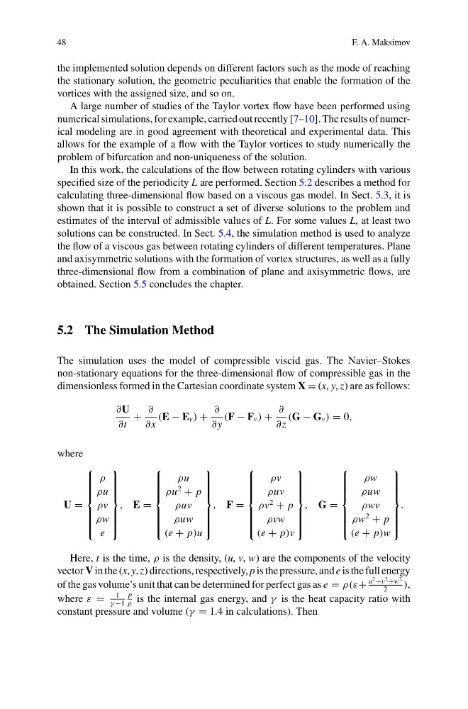
The simulation uses the model of compressible viscid gas. The Navier–Stokes
non-stationary equations for the three-dimensional flow of compressible gas in the
dimensionless formed in the Cartesian coordinate system X = (x, y, z) are as follows:
∂U
∂t
+
∂
∂ x
(E − E v ) +
∂
∂ y
(F − F v ) +
∂
∂z
(G − G v ) = 0,
where
U =
⎧
⎪ ⎪ ⎪ ⎪ ⎪ ⎨
⎪ ⎪ ⎪ ⎪ ⎪ ⎩
ρ
ρu
ρv
ρw
e
⎫
⎪ ⎪ ⎪ ⎪ ⎪ ⎬
⎪ ⎪ ⎪ ⎪ ⎪ ⎭
, E =
⎧
⎪ ⎪ ⎪ ⎪ ⎪ ⎨
⎪ ⎪ ⎪ ⎪ ⎪ ⎩
ρu
ρu
2
+ p
ρuv
ρuw
(e + p)u
⎫
⎪ ⎪ ⎪ ⎪ ⎪ ⎬
⎪ ⎪ ⎪ ⎪ ⎪ ⎭
, F =
⎧
⎪ ⎪ ⎪ ⎪ ⎪ ⎨
⎪ ⎪ ⎪ ⎪ ⎪ ⎩
ρv
ρuv
ρv
2
+ p
ρvw
(e + p)v
⎫
⎪ ⎪ ⎪ ⎪ ⎪ ⎬
⎪ ⎪ ⎪ ⎪ ⎪ ⎭
, G =
⎧
⎪ ⎪ ⎪ ⎪ ⎪ ⎨
⎪ ⎪ ⎪ ⎪ ⎪ ⎩
ρw
ρuw
ρwv
ρw
2
+ p
(e + p)w
⎫
⎪ ⎪ ⎪ ⎪ ⎪ ⎬
⎪ ⎪ ⎪ ⎪ ⎪ ⎭
.
Here, t is the time, ρ is the density, (u, v, w) are the components of the velocity
vector V in the (x, y, z) directions, respectively, p is the pressure, and e is the full energy
of the gas volume’s unit that can be determined for perfect gas as e = ρ(ε+
u
2 +v
2 +w
2
2
),
where ε =
1
γ −1
p
ρ
is the internal gas energy, and γ is the heat capacity ratio with
constant pressure and volume (γ = 1.4 in calculations). Then
F. A. Maksimov
the implemented solution depends on different factors such as the mode of reaching
the stationary solution, the geometric peculiarities that enable the formation of the
vortices with the assigned size, and so on.
A large number of studies of the Taylor vortex flow have been performed using
numerical simulations, for example, carried out recently [7–10]. The results of numerical modeling are in good agreement with theoretical and experimental data. This
allows for the example of a flow with the Taylor vortices to study numerically the
problem of bifurcation and non-uniqueness of the solution.
In this work, the calculations of the flow between rotating cylinders with various
specified size of the periodicity L are performed. Section 5.2 describes a method for
calculating three-dimensional flow based on a viscous gas model. In Sect. 5.3, it is
shown that it is possible to construct a set of diverse solutions to the problem and
estimates of the interval of admissible values of L. For some values L, at least two
solutions can be constructed. In Sect. 5.4, the simulation method is used to analyze
the flow of a viscous gas between rotating cylinders of different temperatures. Plane
and axisymmetric solutions with the formation of vortex structures, as well as a fully
three-dimensional flow from a combination of plane and axisymmetric flows, are
obtained. Section 5.5 concludes the chapter.
5.2 The Simulation Method
The simulation uses the model of compressible viscid gas. The Navier–Stokes
non-stationary equations for the three-dimensional flow of compressible gas in the
dimensionless formed in the Cartesian coordinate system X = (x, y, z) are as follows:
∂U
∂t
+
∂
∂ x
(E − E v ) +
∂
∂ y
(F − F v ) +
∂
∂z
(G − G v ) = 0,
where
U =
⎧
⎪ ⎪ ⎪ ⎪ ⎪ ⎨
⎪ ⎪ ⎪ ⎪ ⎪ ⎩
ρ
ρu
ρv
ρw
e
⎫
⎪ ⎪ ⎪ ⎪ ⎪ ⎬
⎪ ⎪ ⎪ ⎪ ⎪ ⎭
, E =
⎧
⎪ ⎪ ⎪ ⎪ ⎪ ⎨
⎪ ⎪ ⎪ ⎪ ⎪ ⎩
ρu
ρu
2
+ p
ρuv
ρuw
(e + p)u
⎫
⎪ ⎪ ⎪ ⎪ ⎪ ⎬
⎪ ⎪ ⎪ ⎪ ⎪ ⎭
, F =
⎧
⎪ ⎪ ⎪ ⎪ ⎪ ⎨
⎪ ⎪ ⎪ ⎪ ⎪ ⎩
ρv
ρuv
ρv
2
+ p
ρvw
(e + p)v
⎫
⎪ ⎪ ⎪ ⎪ ⎪ ⎬
⎪ ⎪ ⎪ ⎪ ⎪ ⎭
, G =
⎧
⎪ ⎪ ⎪ ⎪ ⎪ ⎨
⎪ ⎪ ⎪ ⎪ ⎪ ⎩
ρw
ρuw
ρwv
ρw
2
+ p
(e + p)w
⎫
⎪ ⎪ ⎪ ⎪ ⎪ ⎬
⎪ ⎪ ⎪ ⎪ ⎪ ⎭
.
Here, t is the time, ρ is the density, (u, v, w) are the components of the velocity
vector V in the (x, y, z) directions, respectively, p is the pressure, and e is the full energy
of the gas volume’s unit that can be determined for perfect gas as e = ρ(ε+
u
2 +v
2 +w
2
2
),
where ε =
1
γ −1
p
ρ
is the internal gas energy, and γ is the heat capacity ratio with
constant pressure and volume (γ = 1.4 in calculations). Then