

364
V. L. Kondarattsev et al.
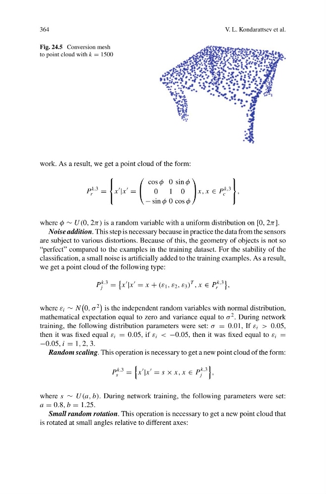
Fig. 24.5 Conversion mesh
to point cloud with k = 1500
work. As a result, we get a point cloud of the form:
P
k.3
r
=
⎧
⎨
⎩
x
|x
=
⎛
⎝
cos φ 0 sin φ
0
1 0
− sin φ 0 cos φ
⎞
⎠ x, x ∈ P
k,3
c
⎫
⎬
⎭
,
where φ ∼ U (0, 2π ) is a random variable with a uniform distribution on [0, 2π ].
Noise addition. This step is necessary because in practice the data from the sensors
are subject to various distortions. Because of this, the geometry of objects is not so
“perfect” compared to the examples in the training dataset. For the stability of the
classification, a small noise is artificially added to the training examples. As a result,
we get a point cloud of the following type:
P
k.3
j
=
x
|x
= x + (ε 1 , ε 2 , ε 3 )
T
, x ∈ P
k,3
r
,
where ε i ∼ N
0, σ
2
is the independent random variables with normal distribution,
mathematical expectation equal to zero and variance equal to σ
2
. During network
training, the following distribution parameters were set: σ = 0.01, If ε i > 0.05,
then it was fixed equal ε i = 0.05, if ε i < −0.05, then it was fixed equal to ε i =
−0.05, i = 1, 2, 3.
Random scaling. This operation is necessary to get a new point cloud of the form:
P
k.3
s
=
x
|x
= s × x, x ∈ P
k,3
j
,
where s ∼ U (a, b). During network training, the following parameters were set:
a = 0.8, b = 1.25.
Small random rotation. This operation is necessary to get a new point cloud that
is rotated at small angles relative to different axes:
V. L. Kondarattsev et al.
Fig. 24.5 Conversion mesh
to point cloud with k = 1500
work. As a result, we get a point cloud of the form:
P
k.3
r
=
⎧
⎨
⎩
x
|x
=
⎛
⎝
cos φ 0 sin φ
0
1 0
− sin φ 0 cos φ
⎞
⎠ x, x ∈ P
k,3
c
⎫
⎬
⎭
,
where φ ∼ U (0, 2π ) is a random variable with a uniform distribution on [0, 2π ].
Noise addition. This step is necessary because in practice the data from the sensors
are subject to various distortions. Because of this, the geometry of objects is not so
“perfect” compared to the examples in the training dataset. For the stability of the
classification, a small noise is artificially added to the training examples. As a result,
we get a point cloud of the following type:
P
k.3
j
=
x
|x
= x + (ε 1 , ε 2 , ε 3 )
T
, x ∈ P
k,3
r
,
where ε i ∼ N
0, σ
2
is the independent random variables with normal distribution,
mathematical expectation equal to zero and variance equal to σ
2
. During network
training, the following distribution parameters were set: σ = 0.01, If ε i > 0.05,
then it was fixed equal ε i = 0.05, if ε i < −0.05, then it was fixed equal to ε i =
−0.05, i = 1, 2, 3.
Random scaling. This operation is necessary to get a new point cloud of the form:
P
k.3
s
=
x
|x
= s × x, x ∈ P
k,3
j
,
where s ∼ U (a, b). During network training, the following parameters were set:
a = 0.8, b = 1.25.
Small random rotation. This operation is necessary to get a new point cloud that
is rotated at small angles relative to different axes: