

24 3D Object Classification, Visual Search …
361
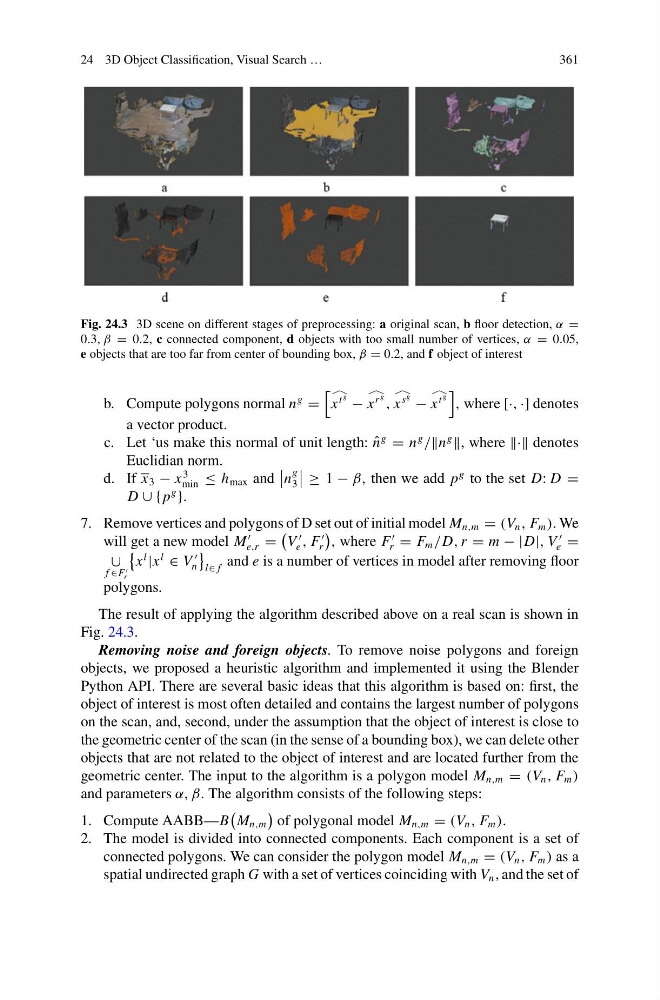
Fig. 24.3 3D scene on different stages of preprocessing: a original scan, b floor detection, α =
0.3, β = 0.2, c connected component, d objects with too small number of vertices, α = 0.05,
e objects that are too far from center of bounding box, β = 0.2, and f object of interest
b. Compute polygons normal n
g
=
x
t
g
− x
r
g
, x
s
g
− x
t
g
, where [·, ·] denotes
a vector product.
c. Let ‘us make this normal of unit length: ˆ
n
g
= n
g
/n
g
, where · denotes
Euclidian norm.
d. If x 3 − x
3
min ≤ h max and
n
g
3
≥ 1 − β, then we add p
g to the set D: D =
D ∪ { p
g
}.
7. Remove vertices and polygons of D set out of initial model M n,m = (V n , F m ). We
will get a new model M
e,r =
V
e , F
r
, where F
r = F m /D, r = m − |D|, V
e =
∪
f ∈F
r
x
l
|x
l
∈ V
n
l∈ f
and e is a number of vertices in model after removing floor
polygons.
The result of applying the algorithm described above on a real scan is shown in
Fig. 24.3.
Removing noise and foreign objects. To remove noise polygons and foreign
objects, we proposed a heuristic algorithm and implemented it using the Blender
Python API. There are several basic ideas that this algorithm is based on: first, the
object of interest is most often detailed and contains the largest number of polygons
on the scan, and, second, under the assumption that the object of interest is close to
the geometric center of the scan (in the sense of a bounding box), we can delete other
objects that are not related to the object of interest and are located further from the
geometric center. The input to the algorithm is a polygon model M n,m = (V n , F m )
and parameters α, β. The algorithm consists of the following steps:
1. Compute AABB—B
M n,m
of polygonal model M n,m = (V n , F m ).
2. The model is divided into connected components. Each component is a set of
connected polygons. We can consider the polygon model M n,m = (V n , F m ) as a
spatial undirected graph G with a set of vertices coinciding with V n , and the set of
361
Fig. 24.3 3D scene on different stages of preprocessing: a original scan, b floor detection, α =
0.3, β = 0.2, c connected component, d objects with too small number of vertices, α = 0.05,
e objects that are too far from center of bounding box, β = 0.2, and f object of interest
b. Compute polygons normal n
g
=
x
t
g
− x
r
g
, x
s
g
− x
t
g
, where [·, ·] denotes
a vector product.
c. Let ‘us make this normal of unit length: ˆ
n
g
= n
g
/n
g
, where · denotes
Euclidian norm.
d. If x 3 − x
3
min ≤ h max and
n
g
3
≥ 1 − β, then we add p
g to the set D: D =
D ∪ { p
g
}.
7. Remove vertices and polygons of D set out of initial model M n,m = (V n , F m ). We
will get a new model M
e,r =
V
e , F
r
, where F
r = F m /D, r = m − |D|, V
e =
∪
f ∈F
r
x
l
|x
l
∈ V
n
l∈ f
and e is a number of vertices in model after removing floor
polygons.
The result of applying the algorithm described above on a real scan is shown in
Fig. 24.3.
Removing noise and foreign objects. To remove noise polygons and foreign
objects, we proposed a heuristic algorithm and implemented it using the Blender
Python API. There are several basic ideas that this algorithm is based on: first, the
object of interest is most often detailed and contains the largest number of polygons
on the scan, and, second, under the assumption that the object of interest is close to
the geometric center of the scan (in the sense of a bounding box), we can delete other
objects that are not related to the object of interest and are located further from the
geometric center. The input to the algorithm is a polygon model M n,m = (V n , F m )
and parameters α, β. The algorithm consists of the following steps:
1. Compute AABB—B
M n,m
of polygonal model M n,m = (V n , F m ).
2. The model is divided into connected components. Each component is a set of
connected polygons. We can consider the polygon model M n,m = (V n , F m ) as a
spatial undirected graph G with a set of vertices coinciding with V n , and the set of