

19 Adaptive Interpolation, TT-Decomposition and Sparse …
281
vertex into two can be more expensive from a computational point of view than
increasing the number of nodes within a single grid.
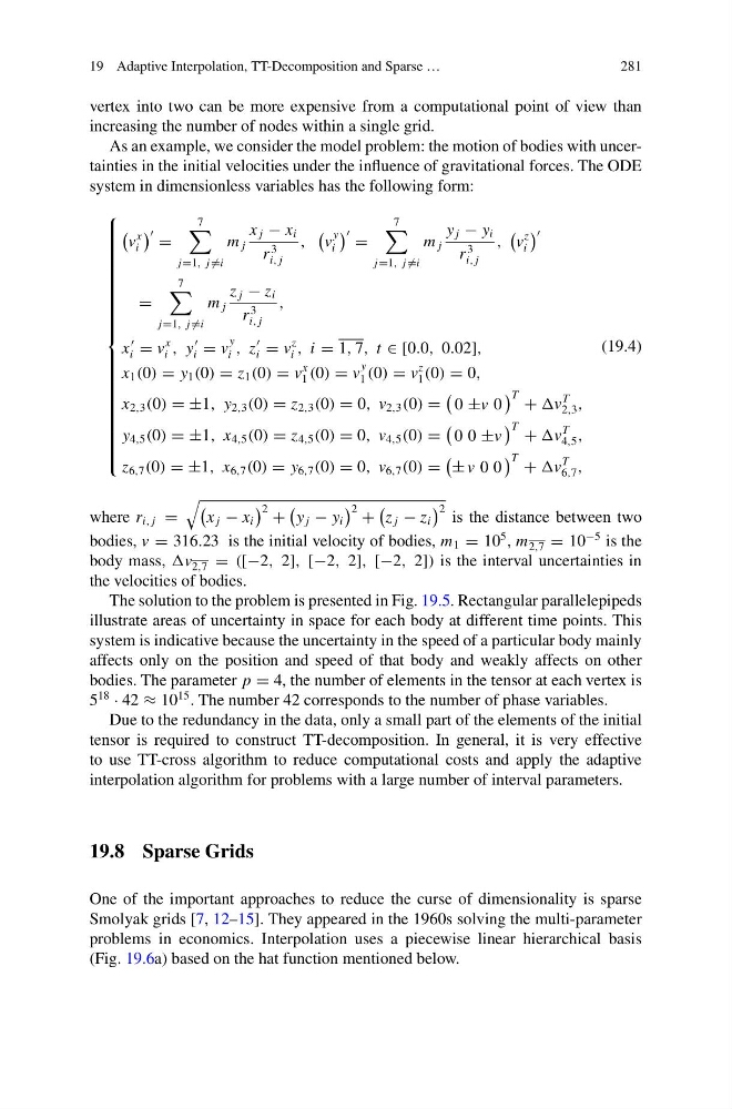
As an example, we consider the model problem: the motion of bodies with uncertainties in the initial velocities under the influence of gravitational forces. The ODE
system in dimensionless variables has the following form:
⎧
⎪ ⎪ ⎪ ⎪ ⎪ ⎪ ⎪ ⎪ ⎪ ⎪ ⎪ ⎪ ⎪ ⎪ ⎪ ⎪ ⎪ ⎪ ⎪ ⎪ ⎨
⎪ ⎪ ⎪ ⎪ ⎪ ⎪ ⎪ ⎪ ⎪ ⎪ ⎪ ⎪ ⎪ ⎪ ⎪ ⎪ ⎪ ⎪ ⎪ ⎪ ⎩
v
x
i
=
7
j=1, j =i
m j
x j − x i
r
3
i, j
,
v
y
i
=
7
j=1, j =i
m j
y j − y i
r
3
i, j
,
v
z
i
=
7
j=1, j =i
m j
z j − z i
r
3
i, j
,
x
i = v
x
i , y
i = v
y
i , z
i = v
z
i , i = 1, 7, t ∈ [0.0, 0.02],
x 1 (0) = y 1 (0) = z 1 (0) = v
x
1 (0) = v
y
1 (0) = v
z
1 (0) = 0,
x 2,3 (0) = ±1, y 2,3 (0) = z 2,3 (0) = 0, v 2,3 (0) =
0 ±v 0
T + v
T
2,3 ,
y 4,5 (0) = ±1, x 4,5 (0) = z 4,5 (0) = 0, v 4,5 (0) =
0 0 ±v
T + v
T
4,5 ,
z 6,7 (0) = ±1, x 6,7 (0) = y 6,7 (0) = 0, v 6,7 (0) =
± v 0 0
T + v
T
6,7 ,
(19.4)
where r i, j =
x j − x i
2 +
y j − y i
2 +
z j − z i
2 is the distance between two
bodies, v = 316.23 is the initial velocity of bodies, m 1 = 10
5 , m 2,7 = 10
−5 is the
body mass, v 2,7 = ([−2, 2], [−2, 2], [−2, 2]) is the interval uncertainties in
the velocities of bodies.
The solution to the problem is presented in Fig. 19.5. Rectangular parallelepipeds
illustrate areas of uncertainty in space for each body at different time points. This
system is indicative because the uncertainty in the speed of a particular body mainly
affects only on the position and speed of that body and weakly affects on other
bodies. The parameter p = 4, the number of elements in the tensor at each vertex is
5
18
· 42 ≈ 10
15 . The number 42 corresponds to the number of phase variables.
Due to the redundancy in the data, only a small part of the elements of the initial
tensor is required to construct TT-decomposition. In general, it is very effective
to use TT-cross algorithm to reduce computational costs and apply the adaptive
interpolation algorithm for problems with a large number of interval parameters.
19.8 Sparse Grids
One of the important approaches to reduce the curse of dimensionality is sparse
Smolyak grids [7, 12–15]. They appeared in the 1960s solving the multi-parameter
problems in economics. Interpolation uses a piecewise linear hierarchical basis
(Fig. 19.6a) based on the hat function mentioned below.
281
vertex into two can be more expensive from a computational point of view than
increasing the number of nodes within a single grid.
As an example, we consider the model problem: the motion of bodies with uncertainties in the initial velocities under the influence of gravitational forces. The ODE
system in dimensionless variables has the following form:
⎧
⎪ ⎪ ⎪ ⎪ ⎪ ⎪ ⎪ ⎪ ⎪ ⎪ ⎪ ⎪ ⎪ ⎪ ⎪ ⎪ ⎪ ⎪ ⎪ ⎪ ⎨
⎪ ⎪ ⎪ ⎪ ⎪ ⎪ ⎪ ⎪ ⎪ ⎪ ⎪ ⎪ ⎪ ⎪ ⎪ ⎪ ⎪ ⎪ ⎪ ⎪ ⎩
v
x
i
=
7
j=1, j =i
m j
x j − x i
r
3
i, j
,
v
y
i
=
7
j=1, j =i
m j
y j − y i
r
3
i, j
,
v
z
i
=
7
j=1, j =i
m j
z j − z i
r
3
i, j
,
x
i = v
x
i , y
i = v
y
i , z
i = v
z
i , i = 1, 7, t ∈ [0.0, 0.02],
x 1 (0) = y 1 (0) = z 1 (0) = v
x
1 (0) = v
y
1 (0) = v
z
1 (0) = 0,
x 2,3 (0) = ±1, y 2,3 (0) = z 2,3 (0) = 0, v 2,3 (0) =
0 ±v 0
T + v
T
2,3 ,
y 4,5 (0) = ±1, x 4,5 (0) = z 4,5 (0) = 0, v 4,5 (0) =
0 0 ±v
T + v
T
4,5 ,
z 6,7 (0) = ±1, x 6,7 (0) = y 6,7 (0) = 0, v 6,7 (0) =
± v 0 0
T + v
T
6,7 ,
(19.4)
where r i, j =
x j − x i
2 +
y j − y i
2 +
z j − z i
2 is the distance between two
bodies, v = 316.23 is the initial velocity of bodies, m 1 = 10
5 , m 2,7 = 10
−5 is the
body mass, v 2,7 = ([−2, 2], [−2, 2], [−2, 2]) is the interval uncertainties in
the velocities of bodies.
The solution to the problem is presented in Fig. 19.5. Rectangular parallelepipeds
illustrate areas of uncertainty in space for each body at different time points. This
system is indicative because the uncertainty in the speed of a particular body mainly
affects only on the position and speed of that body and weakly affects on other
bodies. The parameter p = 4, the number of elements in the tensor at each vertex is
5
18
· 42 ≈ 10
15 . The number 42 corresponds to the number of phase variables.
Due to the redundancy in the data, only a small part of the elements of the initial
tensor is required to construct TT-decomposition. In general, it is very effective
to use TT-cross algorithm to reduce computational costs and apply the adaptive
interpolation algorithm for problems with a large number of interval parameters.
19.8 Sparse Grids
One of the important approaches to reduce the curse of dimensionality is sparse
Smolyak grids [7, 12–15]. They appeared in the 1960s solving the multi-parameter
problems in economics. Interpolation uses a piecewise linear hierarchical basis
(Fig. 19.6a) based on the hat function mentioned below.