

19 Adaptive Interpolation, TT-Decomposition and Sparse …
273
⎧
⎪ ⎪ ⎪ ⎪ ⎪ ⎪ ⎨
⎪ ⎪ ⎪ ⎪ ⎪ ⎪ ⎩
dx i (t)
dt
= f i (x 1 (t), x 2 (t), . . . , x n (t)) i = 1, n
x i (t 0 ) ∈
x
0
i , x
0
i
i = 1, m
x i (t 0 ) = x
0
i i = m + 1, n
t ∈ [t 0 , t N ]
(19.1)
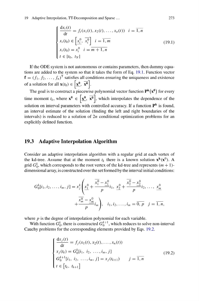
If the ODE system is not autonomous or contains parameters, then dummy equations are added to the system so that it takes the form of Eq. 19.1. Function vector
f = ( f 1 , f 2 , . . . , f n )
T satisfies all conditions ensuring the uniqueness and existence
of a solution for all x(t 0 ) ∈
x
0
, x 0
.
The goal is to construct a piecewise polynomial vector function P
k
x
0
for every
time moment t k , where x
0
∈
x
0
, x 0
, which interpolates the dependence of the
solution on interval parameters with controlled accuracy. If a function P
k is found,
an interval estimate of the solution (finding the left and right boundaries of the
intervals) is reduced to a solution of 2n conditional optimization problems for an
explicitly defined function.
19.3 Adaptive Interpolation Algorithm
Consider an adaptive interpolation algorithm with a regular grid at each vertex of
the kd-tree. Assume that at the moment t k there is a known solution x
k
(x
0
). A
grid G
k
0 , which corresponds to the root vertex of the kd-tree and represents (m + 1)dimensional array, is constructed over the set formed by the interval initial conditions:
G
k
0 [i 1 , i 2 , . . . , i m , j] = x
k
j
⎛
⎝ x
0
1 +
x
0
1 − x
0
1
p
i 1 , x
0
2 +
x
0
2 − x
0
2
p
i 2 , . . . , x
0
m
+
x 0
m − x
0
m
p
i m
, i 1 , i 2 , . . . , i m = 0, p j = 1, n,
where p is the degree of interpolation polynomial for each variable.
With function G
k
0 , there is constructed G
k+1
0 , which reduces to solve non-interval
Cauchy problems for the corresponding elements provided by Eqs. 19.2.
⎧
⎪ ⎪ ⎪ ⎪ ⎪ ⎨
⎪ ⎪ ⎪ ⎪ ⎪ ⎩
dx j (t)
dt
= f j (x 1 (t), x 2 (t), . . . , x n (t))
x j (t k ) = G
k
0 [i 1 , i 2 , . . . , i m , j]
G
k+1
0 [i 1 , i 2 , . . . , i m , j] = x j (t k+1 )
j = 1, n
t ∈
t k , t k+1
(19.2)
273
⎧
⎪ ⎪ ⎪ ⎪ ⎪ ⎪ ⎨
⎪ ⎪ ⎪ ⎪ ⎪ ⎪ ⎩
dx i (t)
dt
= f i (x 1 (t), x 2 (t), . . . , x n (t)) i = 1, n
x i (t 0 ) ∈
x
0
i , x
0
i
i = 1, m
x i (t 0 ) = x
0
i i = m + 1, n
t ∈ [t 0 , t N ]
(19.1)
If the ODE system is not autonomous or contains parameters, then dummy equations are added to the system so that it takes the form of Eq. 19.1. Function vector
f = ( f 1 , f 2 , . . . , f n )
T satisfies all conditions ensuring the uniqueness and existence
of a solution for all x(t 0 ) ∈
x
0
, x 0
.
The goal is to construct a piecewise polynomial vector function P
k
x
0
for every
time moment t k , where x
0
∈
x
0
, x 0
, which interpolates the dependence of the
solution on interval parameters with controlled accuracy. If a function P
k is found,
an interval estimate of the solution (finding the left and right boundaries of the
intervals) is reduced to a solution of 2n conditional optimization problems for an
explicitly defined function.
19.3 Adaptive Interpolation Algorithm
Consider an adaptive interpolation algorithm with a regular grid at each vertex of
the kd-tree. Assume that at the moment t k there is a known solution x
k
(x
0
). A
grid G
k
0 , which corresponds to the root vertex of the kd-tree and represents (m + 1)dimensional array, is constructed over the set formed by the interval initial conditions:
G
k
0 [i 1 , i 2 , . . . , i m , j] = x
k
j
⎛
⎝ x
0
1 +
x
0
1 − x
0
1
p
i 1 , x
0
2 +
x
0
2 − x
0
2
p
i 2 , . . . , x
0
m
+
x 0
m − x
0
m
p
i m
, i 1 , i 2 , . . . , i m = 0, p j = 1, n,
where p is the degree of interpolation polynomial for each variable.
With function G
k
0 , there is constructed G
k+1
0 , which reduces to solve non-interval
Cauchy problems for the corresponding elements provided by Eqs. 19.2.
⎧
⎪ ⎪ ⎪ ⎪ ⎪ ⎨
⎪ ⎪ ⎪ ⎪ ⎪ ⎩
dx j (t)
dt
= f j (x 1 (t), x 2 (t), . . . , x n (t))
x j (t k ) = G
k
0 [i 1 , i 2 , . . . , i m , j]
G
k+1
0 [i 1 , i 2 , . . . , i m , j] = x j (t k+1 )
j = 1, n
t ∈
t k , t k+1
(19.2)