

17 Modified Continuous-Time Particle Filter Algorithm …
255
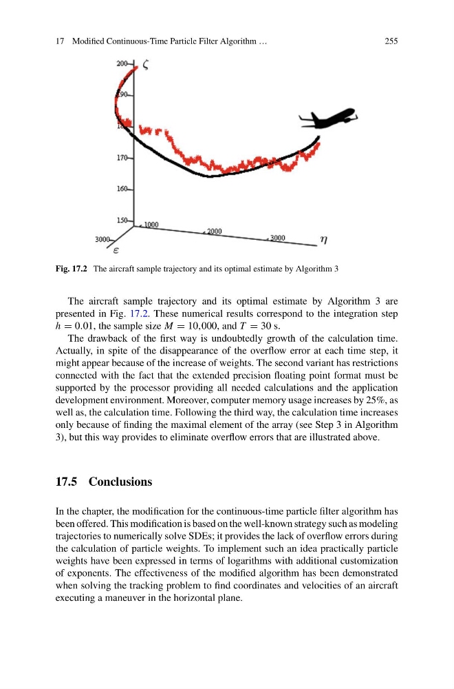
Fig. 17.2 The aircraft sample trajectory and its optimal estimate by Algorithm 3
The aircraft sample trajectory and its optimal estimate by Algorithm 3 are
presented in Fig. 17.2. These numerical results correspond to the integration step
h = 0.01, the sample size M = 10,000, and T = 30 s.
The drawback of the first way is undoubtedly growth of the calculation time.
Actually, in spite of the disappearance of the overflow error at each time step, it
might appear because of the increase of weights. The second variant has restrictions
connected with the fact that the extended precision floating point format must be
supported by the processor providing all needed calculations and the application
development environment. Moreover, computer memory usage increases by 25%, as
well as, the calculation time. Following the third way, the calculation time increases
only because of finding the maximal element of the array (see Step 3 in Algorithm
3), but this way provides to eliminate overflow errors that are illustrated above.
17.5 Conclusions
In the chapter, the modification for the continuous-time particle filter algorithm has
been offered. This modification is based on the well-known strategy such as modeling
trajectories to numerically solve SDEs; it provides the lack of overflow errors during
the calculation of particle weights. To implement such an idea practically particle
weights have been expressed in terms of logarithms with additional customization
of exponents. The effectiveness of the modified algorithm has been demonstrated
when solving the tracking problem to find coordinates and velocities of an aircraft
executing a maneuver in the horizontal plane.
255
Fig. 17.2 The aircraft sample trajectory and its optimal estimate by Algorithm 3
The aircraft sample trajectory and its optimal estimate by Algorithm 3 are
presented in Fig. 17.2. These numerical results correspond to the integration step
h = 0.01, the sample size M = 10,000, and T = 30 s.
The drawback of the first way is undoubtedly growth of the calculation time.
Actually, in spite of the disappearance of the overflow error at each time step, it
might appear because of the increase of weights. The second variant has restrictions
connected with the fact that the extended precision floating point format must be
supported by the processor providing all needed calculations and the application
development environment. Moreover, computer memory usage increases by 25%, as
well as, the calculation time. Following the third way, the calculation time increases
only because of finding the maximal element of the array (see Step 3 in Algorithm
3), but this way provides to eliminate overflow errors that are illustrated above.
17.5 Conclusions
In the chapter, the modification for the continuous-time particle filter algorithm has
been offered. This modification is based on the well-known strategy such as modeling
trajectories to numerically solve SDEs; it provides the lack of overflow errors during
the calculation of particle weights. To implement such an idea practically particle
weights have been expressed in terms of logarithms with additional customization
of exponents. The effectiveness of the modified algorithm has been demonstrated
when solving the tracking problem to find coordinates and velocities of an aircraft
executing a maneuver in the horizontal plane.