

17 Modified Continuous-Time Particle Filter Algorithm …
253
problem. The developed software has been tested on the tracking problem described
in the next section.
17.4 Simulations
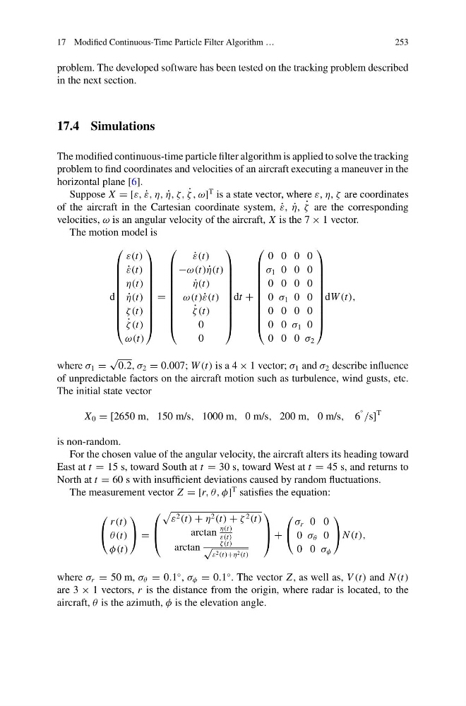
The modified continuous-time particle filter algorithm is applied to solve the tracking
problem to find coordinates and velocities of an aircraft executing a maneuver in the
horizontal plane [6].
Suppose X = [ε, ˙
ε, η, ˙
η, ζ, ˙
ζ , ω]
T is a state vector, where ε, η, ζ are coordinates
of the aircraft in the Cartesian coordinate system, ˙
ε, ˙
η, ˙
ζ are the corresponding
velocities, ω is an angular velocity of the aircraft, X is the 7 × 1 vector.
The motion model is
d
⎛
⎜
⎜
⎜
⎜
⎜
⎜
⎜
⎜
⎜
⎝
ε(t)
˙
ε(t)
η(t)
˙
η(t)
ζ(t)
˙
ζ (t)
ω(t)
⎞
⎟
⎟
⎟
⎟
⎟
⎟
⎟
⎟
⎟
⎠
=
⎛
⎜
⎜
⎜
⎜
⎜
⎜
⎜
⎜
⎜
⎝
˙
ε(t)
−ω(t) ˙
η(t)
˙
η(t)
ω(t)˙ ε(t)
˙
ζ (t)
0
0
⎞
⎟
⎟
⎟
⎟
⎟
⎟
⎟
⎟
⎟
⎠
dt +
⎛
⎜
⎜
⎜
⎜
⎜
⎜
⎜
⎜
⎜
⎝
0
σ 1
0
0
0
0
0
0
0
0
σ 1
0
0
0
0
0
0
0
0
σ 1
0
0
0
0
0
0
0
σ 2
⎞
⎟
⎟
⎟
⎟
⎟
⎟
⎟
⎟
⎟
⎠
dW (t),
where σ 1 =
√
0.2, σ 2 = 0.007; W (t) is a 4 × 1 vector; σ 1 and σ 2 describe influence
of unpredictable factors on the aircraft motion such as turbulence, wind gusts, etc.
The initial state vector
X 0 = [2650 m, 150 m/s, 1000 m, 0 m/s, 200 m, 0 m/s, 6
◦ /s]
T
is non-random.
For the chosen value of the angular velocity, the aircraft alters its heading toward
East at t = 15 s, toward South at t = 30 s, toward West at t = 45 s, and returns to
North at t = 60 s with insufficient deviations caused by random fluctuations.
The measurement vector Z = [r, θ, φ]
T satisfies the equation:
⎛
⎝
r (t)
θ(t)
φ(t)
⎞
⎠ =
⎛
⎜
⎝
ε 2 (t) + η 2 (t) + ζ 2 (t)
arctan
η(t)
ε(t)
arctan
ζ(t)
√
ε 2 (t)+η 2 (t)
⎞
⎟
⎠ +
⎛
⎝
σ r
0
0
0
σ θ
0
0
0
σ φ
⎞
⎠ N (t),
where σ r = 50 m, σ θ = 0.1
◦ , σ φ = 0.1
◦ . The vector Z , as well as, V (t) and N (t)
are 3 × 1 vectors, r is the distance from the origin, where radar is located, to the
aircraft, θ is the azimuth, φ is the elevation angle.
253
problem. The developed software has been tested on the tracking problem described
in the next section.
17.4 Simulations
The modified continuous-time particle filter algorithm is applied to solve the tracking
problem to find coordinates and velocities of an aircraft executing a maneuver in the
horizontal plane [6].
Suppose X = [ε, ˙
ε, η, ˙
η, ζ, ˙
ζ , ω]
T is a state vector, where ε, η, ζ are coordinates
of the aircraft in the Cartesian coordinate system, ˙
ε, ˙
η, ˙
ζ are the corresponding
velocities, ω is an angular velocity of the aircraft, X is the 7 × 1 vector.
The motion model is
d
⎛
⎜
⎜
⎜
⎜
⎜
⎜
⎜
⎜
⎜
⎝
ε(t)
˙
ε(t)
η(t)
˙
η(t)
ζ(t)
˙
ζ (t)
ω(t)
⎞
⎟
⎟
⎟
⎟
⎟
⎟
⎟
⎟
⎟
⎠
=
⎛
⎜
⎜
⎜
⎜
⎜
⎜
⎜
⎜
⎜
⎝
˙
ε(t)
−ω(t) ˙
η(t)
˙
η(t)
ω(t)˙ ε(t)
˙
ζ (t)
0
0
⎞
⎟
⎟
⎟
⎟
⎟
⎟
⎟
⎟
⎟
⎠
dt +
⎛
⎜
⎜
⎜
⎜
⎜
⎜
⎜
⎜
⎜
⎝
0
σ 1
0
0
0
0
0
0
0
0
σ 1
0
0
0
0
0
0
0
0
σ 1
0
0
0
0
0
0
0
σ 2
⎞
⎟
⎟
⎟
⎟
⎟
⎟
⎟
⎟
⎟
⎠
dW (t),
where σ 1 =
√
0.2, σ 2 = 0.007; W (t) is a 4 × 1 vector; σ 1 and σ 2 describe influence
of unpredictable factors on the aircraft motion such as turbulence, wind gusts, etc.
The initial state vector
X 0 = [2650 m, 150 m/s, 1000 m, 0 m/s, 200 m, 0 m/s, 6
◦ /s]
T
is non-random.
For the chosen value of the angular velocity, the aircraft alters its heading toward
East at t = 15 s, toward South at t = 30 s, toward West at t = 45 s, and returns to
North at t = 60 s with insufficient deviations caused by random fluctuations.
The measurement vector Z = [r, θ, φ]
T satisfies the equation:
⎛
⎝
r (t)
θ(t)
φ(t)
⎞
⎠ =
⎛
⎜
⎝
ε 2 (t) + η 2 (t) + ζ 2 (t)
arctan
η(t)
ε(t)
arctan
ζ(t)
√
ε 2 (t)+η 2 (t)
⎞
⎟
⎠ +
⎛
⎝
σ r
0
0
0
σ θ
0
0
0
σ φ
⎞
⎠ N (t),
where σ r = 50 m, σ θ = 0.1
◦ , σ φ = 0.1
◦ . The vector Z , as well as, V (t) and N (t)
are 3 × 1 vectors, r is the distance from the origin, where radar is located, to the
aircraft, θ is the azimuth, φ is the elevation angle.