

248
I. A. Kudryavtseva and K. A. Rybakov
As a rule, to simulate an ensemble of trajectories and corresponding weights
the numerical methods for solving SDEs are employed. Both the simple method
such as the Euler–Maruyama method having low order of convergence as a result
that leads to low accuracy and methods of a higher order of convergence including
those that possess the additional stability properties can be used [25–27]. If the
filtering problem is needed to solve on manifolds [28–30], the specific modification
of numerical methods given in [31, 32] should be applied.
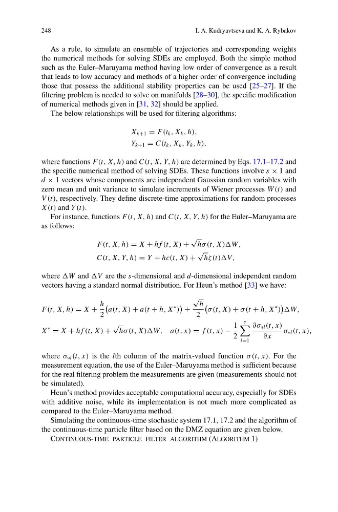
The below relationships will be used for filtering algorithms:
X k+1 = F(t k , X k , h),
Y k+1 = C(t k , X k , Y k , h),
where functions F(t, X, h) and C(t, X, Y, h) are determined by Eqs. 17.1–17.2 and
the specific numerical method of solving SDEs. These functions involve s × 1 and
d × 1 vectors whose components are independent Gaussian random variables with
zero mean and unit variance to simulate increments of Wiener processes W (t) and
V (t), respectively. They define discrete-time approximations for random processes
X (t) and Y (t).
For instance, functions F(t, X, h) and C(t, X, Y, h) for the Euler–Maruyama are
as follows:
F(t, X, h) = X + h f (t, X ) +
√
hσ (t, X ))W,
C(t, X, Y, h) = Y + hc(t, X ) +
√
hζ(t))V,
where W and V are the s-dimensional and d-dimensional independent random
vectors having a standard normal distribution. For Heun’s method [33] we have:
F(t, X, h) = X +
h
2
a(t, X ) + a(t + h, X
∗
)
+
√
h
2
σ (t, X ) + σ (t + h, X
∗
)
W,
X
∗
= X + h f (t, X ) +
√
hσ (t, X ))W, a(t, x) = f (t, x) −
1
2
s
l=1
∂σ ∗l (t, x)
∂ x
σ ∗l (t, x),
where σ ∗l (t, x) is the lth column of the matrix-valued function σ (t, x). For the
measurement equation, the use of the Euler–Maruyama method is sufficient because
for the real filtering problem the measurements are given (measurements should not
be simulated).
Heun’s method provides acceptable computational accuracy, especially for SDEs
with additive noise, while its implementation is not much more complicated as
compared to the Euler–Maruyama method.
Simulating the continuous-time stochastic system 17.1, 17.2 and the algorithm of
the continuous-time particle filter based on the DMZ equation are given below.
Continuous-time particle filter algorithm (Algorithm 1)
I. A. Kudryavtseva and K. A. Rybakov
As a rule, to simulate an ensemble of trajectories and corresponding weights
the numerical methods for solving SDEs are employed. Both the simple method
such as the Euler–Maruyama method having low order of convergence as a result
that leads to low accuracy and methods of a higher order of convergence including
those that possess the additional stability properties can be used [25–27]. If the
filtering problem is needed to solve on manifolds [28–30], the specific modification
of numerical methods given in [31, 32] should be applied.
The below relationships will be used for filtering algorithms:
X k+1 = F(t k , X k , h),
Y k+1 = C(t k , X k , Y k , h),
where functions F(t, X, h) and C(t, X, Y, h) are determined by Eqs. 17.1–17.2 and
the specific numerical method of solving SDEs. These functions involve s × 1 and
d × 1 vectors whose components are independent Gaussian random variables with
zero mean and unit variance to simulate increments of Wiener processes W (t) and
V (t), respectively. They define discrete-time approximations for random processes
X (t) and Y (t).
For instance, functions F(t, X, h) and C(t, X, Y, h) for the Euler–Maruyama are
as follows:
F(t, X, h) = X + h f (t, X ) +
√
hσ (t, X ))W,
C(t, X, Y, h) = Y + hc(t, X ) +
√
hζ(t))V,
where W and V are the s-dimensional and d-dimensional independent random
vectors having a standard normal distribution. For Heun’s method [33] we have:
F(t, X, h) = X +
h
2
a(t, X ) + a(t + h, X
∗
)
+
√
h
2
σ (t, X ) + σ (t + h, X
∗
)
W,
X
∗
= X + h f (t, X ) +
√
hσ (t, X ))W, a(t, x) = f (t, x) −
1
2
s
l=1
∂σ ∗l (t, x)
∂ x
σ ∗l (t, x),
where σ ∗l (t, x) is the lth column of the matrix-valued function σ (t, x). For the
measurement equation, the use of the Euler–Maruyama method is sufficient because
for the real filtering problem the measurements are given (measurements should not
be simulated).
Heun’s method provides acceptable computational accuracy, especially for SDEs
with additive noise, while its implementation is not much more complicated as
compared to the Euler–Maruyama method.
Simulating the continuous-time stochastic system 17.1, 17.2 and the algorithm of
the continuous-time particle filter based on the DMZ equation are given below.
Continuous-time particle filter algorithm (Algorithm 1)