

208
S. S. Krylov et al.
Even the regular tidal potential [16], due to the complexity of the topography
of the global ocean floor and contours of the continents coastlines, leads to the
development of a random displacement field and occurrence of random fluctuations
in tidal processes. These perturbations correspond to weak irregular perturbations
of the Earth’s inertia tensor components. However, due to the uneven distribution of
the global ocean’s water masses over the Earth’s surface, their manifestation in the
centrifugal moments of inertia J xz , J yz , and, therefore, in the coordinates x p , y p , are
different.
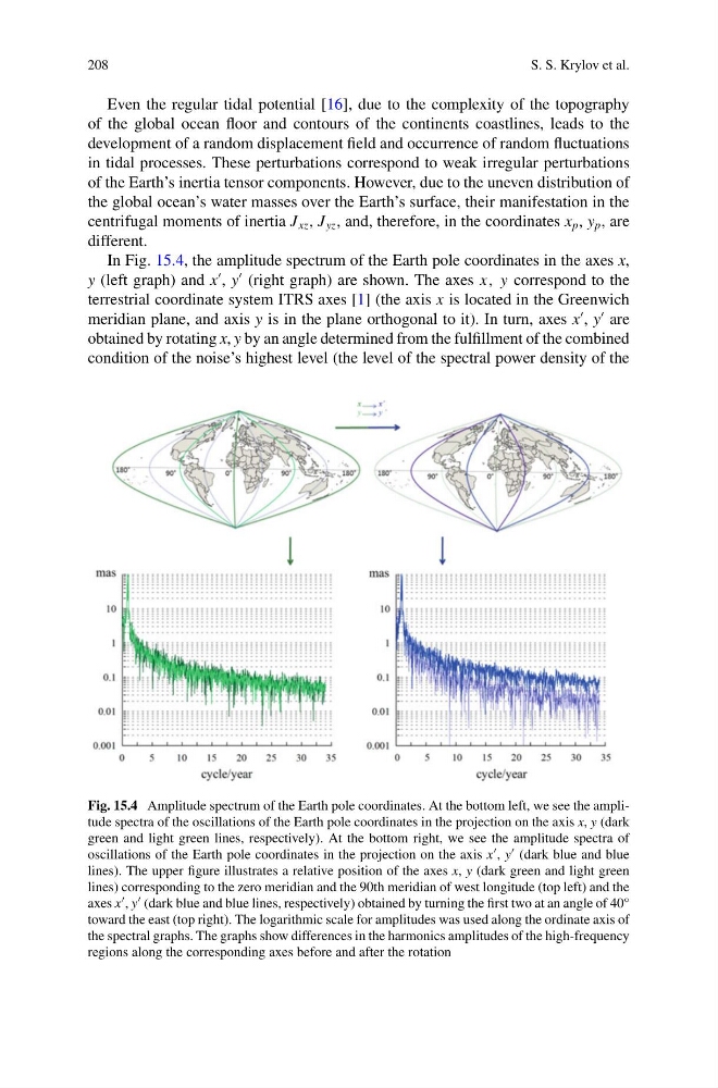
In Fig. 15.4, the amplitude spectrum of the Earth pole coordinates in the axes x,
y (left graph) and x
, y
(right graph) are shown. The axes x, y correspond to the
terrestrial coordinate system ITRS axes [1] (the axis x is located in the Greenwich
meridian plane, and axis y is in the plane orthogonal to it). In turn, axes x
, y
are
obtained by rotating x, y by an angle determined from the fulfillment of the combined
condition of the noise’s highest level (the level of the spectral power density of the
Fig. 15.4 Amplitude spectrum of the Earth pole coordinates. At the bottom left, we see the amplitude spectra of the oscillations of the Earth pole coordinates in the projection on the axis x, y (dark
green and light green lines, respectively). At the bottom right, we see the amplitude spectra of
oscillations of the Earth pole coordinates in the projection on the axis x , y (dark blue and blue
lines). The upper figure illustrates a relative position of the axes x, y (dark green and light green
lines) corresponding to the zero meridian and the 90th meridian of west longitude (top left) and the
axes x , y (dark blue and blue lines, respectively) obtained by turning the first two at an angle of 40°
toward the east (top right). The logarithmic scale for amplitudes was used along the ordinate axis of
the spectral graphs. The graphs show differences in the harmonics amplitudes of the high-frequency
regions along the corresponding axes before and after the rotation
S. S. Krylov et al.
Even the regular tidal potential [16], due to the complexity of the topography
of the global ocean floor and contours of the continents coastlines, leads to the
development of a random displacement field and occurrence of random fluctuations
in tidal processes. These perturbations correspond to weak irregular perturbations
of the Earth’s inertia tensor components. However, due to the uneven distribution of
the global ocean’s water masses over the Earth’s surface, their manifestation in the
centrifugal moments of inertia J xz , J yz , and, therefore, in the coordinates x p , y p , are
different.
In Fig. 15.4, the amplitude spectrum of the Earth pole coordinates in the axes x,
y (left graph) and x
, y
(right graph) are shown. The axes x, y correspond to the
terrestrial coordinate system ITRS axes [1] (the axis x is located in the Greenwich
meridian plane, and axis y is in the plane orthogonal to it). In turn, axes x
, y
are
obtained by rotating x, y by an angle determined from the fulfillment of the combined
condition of the noise’s highest level (the level of the spectral power density of the
Fig. 15.4 Amplitude spectrum of the Earth pole coordinates. At the bottom left, we see the amplitude spectra of the oscillations of the Earth pole coordinates in the projection on the axis x, y (dark
green and light green lines, respectively). At the bottom right, we see the amplitude spectra of
oscillations of the Earth pole coordinates in the projection on the axis x , y (dark blue and blue
lines). The upper figure illustrates a relative position of the axes x, y (dark green and light green
lines) corresponding to the zero meridian and the 90th meridian of west longitude (top left) and the
axes x , y (dark blue and blue lines, respectively) obtained by turning the first two at an angle of 40°
toward the east (top right). The logarithmic scale for amplitudes was used along the ordinate axis of
the spectral graphs. The graphs show differences in the harmonics amplitudes of the high-frequency
regions along the corresponding axes before and after the rotation