

8.13 Calculating Losses Along a Duct Using the Integral Method
337
C 2 = −
π
√
3
− r
2θ
r
2
3
L
4th Calculation of z at the location of the fan (x = 0). Having obtained the value
of the integration constants, Eq. 8.54, which is only dependent on z, can be solved
by numerical methods or using the Excel Solver function.
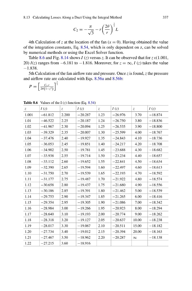
Table 8.6 and Fig. 8.14 shows I (z) versus z. It can be observed that for z ε(1.001,
20) I(z) ranges from −6.181 to −1.816. Moreover, for z = ∞, I (z) takes the value
−1.838.
5th Calculation of the fan airflow rate and pressure. Once z is found, z the pressure
and airflow rate are calculated with Eqs. 8.56a and 8.56b:
P =
C 1 r
2θ(1−z 3 )
2
3
Table 8.6 Values of the I (z) function (Eq. 8.54)
z
I (z)
z
I (z)
z
I (z)
z
I (z)
1.001
−61.812
2.200
−20.287
1.23
−26.976
3.70
−18.874
1.01
−46.522
2.25
−20.187
1.24
−26.750
3.80
−18.836
1.02
−41.967
2.30
−20.094
1.25
−26.535
3.90
−18.800
1.03
−39.329
2.35
−20.007
1.30
−25.599
4.00
−18.767
1.04
−37.476
2.40
−19.927
1.35
−24.843
4.10
−18.736
1.05
−36.053
2.45
−19.851
1.40
−24.217
4.20
−18.708
1.06
−34.902
2.50
−19.781
1.45
−23.688
4.30
−18.682
1.07
−33.938
2.55
−19.714
1.50
−23.234
4.40
−18.657
1.08
−33.112
2.60
−19.652
1.55
−22.841
4.50
−18.634
1.09
−32.390
2.65
−19.594
1.60
−22.497
4.60
−18.613
1.10
−31.750
2.70
−19.539
1.65
−22.193
4.70
−18.592
1.11
−31.177
2.75
−19.487
1.70
−21.922
4.80
−18.574
1.12
−30.658
2.80
−19.437
1.75
−21.680
4.90
−18.556
1.13
−30.186
2.85
−19.391
1.80
−21.462
5.00
−18.539
1.14
−29.753
2.90
−19.347
1.85
−21.265
6.00
−18.416
1.15
−29.354
2.95
−19.305
1.90
−21.086
7.00
−18.342
1.16
−28.984
3.00
−19.266
1.95
−20.923
8.00
−18.294
1.17
−28.640
3.10
−19.193
2.00
−20.774
9.00
−18.262
1.18
−28.318
3.20
−19.127
2.05
−20.637
10.00
−18.238
1.19
−28.017
3.30
−19.067
2.10
−20.511
15.00
−18.182
1.20
−27.734
3.40
−19.012
2.15
−20.394
20.00
−18.163
1.21
−27.467
3.50
−18.962
2.20
−20.287
∞
−18.138
1.22
−27.215
3.60
−18.916
337
C 2 = −
π
√
3
− r
2θ
r
2
3
L
4th Calculation of z at the location of the fan (x = 0). Having obtained the value
of the integration constants, Eq. 8.54, which is only dependent on z, can be solved
by numerical methods or using the Excel Solver function.
Table 8.6 and Fig. 8.14 shows I (z) versus z. It can be observed that for z ε(1.001,
20) I(z) ranges from −6.181 to −1.816. Moreover, for z = ∞, I (z) takes the value
−1.838.
5th Calculation of the fan airflow rate and pressure. Once z is found, z the pressure
and airflow rate are calculated with Eqs. 8.56a and 8.56b:
P =
C 1 r
2θ(1−z 3 )
2
3
Table 8.6 Values of the I (z) function (Eq. 8.54)
z
I (z)
z
I (z)
z
I (z)
z
I (z)
1.001
−61.812
2.200
−20.287
1.23
−26.976
3.70
−18.874
1.01
−46.522
2.25
−20.187
1.24
−26.750
3.80
−18.836
1.02
−41.967
2.30
−20.094
1.25
−26.535
3.90
−18.800
1.03
−39.329
2.35
−20.007
1.30
−25.599
4.00
−18.767
1.04
−37.476
2.40
−19.927
1.35
−24.843
4.10
−18.736
1.05
−36.053
2.45
−19.851
1.40
−24.217
4.20
−18.708
1.06
−34.902
2.50
−19.781
1.45
−23.688
4.30
−18.682
1.07
−33.938
2.55
−19.714
1.50
−23.234
4.40
−18.657
1.08
−33.112
2.60
−19.652
1.55
−22.841
4.50
−18.634
1.09
−32.390
2.65
−19.594
1.60
−22.497
4.60
−18.613
1.10
−31.750
2.70
−19.539
1.65
−22.193
4.70
−18.592
1.11
−31.177
2.75
−19.487
1.70
−21.922
4.80
−18.574
1.12
−30.658
2.80
−19.437
1.75
−21.680
4.90
−18.556
1.13
−30.186
2.85
−19.391
1.80
−21.462
5.00
−18.539
1.14
−29.753
2.90
−19.347
1.85
−21.265
6.00
−18.416
1.15
−29.354
2.95
−19.305
1.90
−21.086
7.00
−18.342
1.16
−28.984
3.00
−19.266
1.95
−20.923
8.00
−18.294
1.17
−28.640
3.10
−19.193
2.00
−20.774
9.00
−18.262
1.18
−28.318
3.20
−19.127
2.05
−20.637
10.00
−18.238
1.19
−28.017
3.30
−19.067
2.10
−20.511
15.00
−18.182
1.20
−27.734
3.40
−19.012
2.15
−20.394
20.00
−18.163
1.21
−27.467
3.50
−18.962
2.20
−20.287
∞
−18.138
1.22
−27.215
3.60
−18.916