

156
4 Mine Ventilation Networks
Node
Equation
Substituted variable
N 1
Q a + Q 14 = Q 12
Q 14 = Q 12 − Q a
N 3
Q 23 = Q a + Q 34
Q 34 = Q 23 − Q a
N 2
Q 12 = Q 24 + Q 23
Q 24 = Q 12 − Q 23
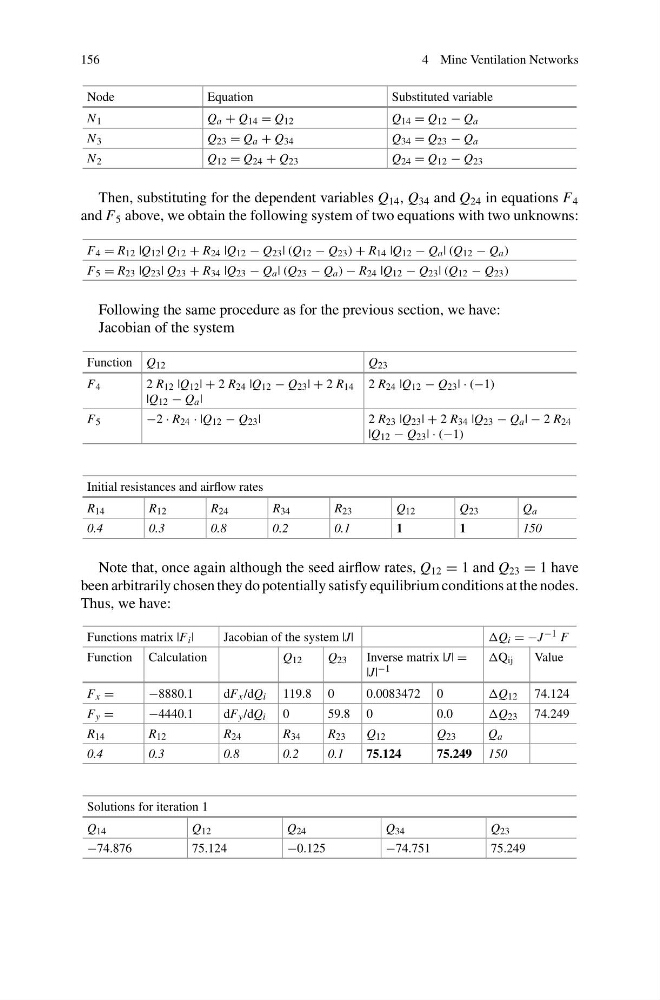
Then, substituting for the dependent variables Q 14 , Q 34 and Q 24 in equations F 4
and F 5 above, we obtain the following system of two equations with two unknowns:
F 4 = R 12 |Q 12 | Q 12 + R 24 |Q 12 − Q 23 | (Q 12 − Q 23 ) + R 14 |Q 12 − Q a | (Q 12 − Q a )
F 5 = R 23 |Q 23 | Q 23 + R 34 |Q 23 − Q a | (Q 23 − Q a ) − R 24 |Q 12 − Q 23 | (Q 12 − Q 23 )
Following the same procedure as for the previous section, we have:
Jacobian of the system
Function Q 12
Q 23
F 4
2 R 12 |Q 12 | + 2 R 24 |Q 12 − Q 23 | + 2 R 14
|Q 12 − Q a |
2 R 24 |Q 12 − Q 23 | · (−1)
F 5
−2 · R 24 · |Q 12 − Q 23 |
2 R 23 |Q 23 | + 2 R 34 |Q 23 − Q a | − 2 R 24
|Q 12 − Q 23 | · (−1)
Initial resistances and airflow rates
R 14
R 12
R 24
R 34
R 23
Q 12
Q 23
Q a
0.4
0.3
0.8
0.2
0.1
1
1
150
Note that, once again although the seed airflow rates, Q 12 = 1 and Q 23 = 1 have
been arbitrarily chosen they do potentially satisfy equilibrium conditions at the nodes.
Thus, we have:
Functions matrix |F i |
Jacobian of the system |J|
Q i = −J −1 F
Function Calculation
Q 12
Q 23
Inverse matrix |J| =
|J| −1
Q ij
Value
F x =
−8880.1
dF x /dQ i 119.8 0
0.0083472 0
Q 12 74.124
F y =
−4440.1
dF y /dQ i 0
59.8 0
0.0
Q 23 74.249
R 14
R 12
R 24
R 34
R 23
Q 12
Q 23
Q a
0.4
0.3
0.8
0.2
0.1
75.124
75.249 150
Solutions for iteration 1
Q 14
Q 12
Q 24
Q 34
Q 23
−74.876
75.124
−0.125
−74.751
75.249
4 Mine Ventilation Networks
Node
Equation
Substituted variable
N 1
Q a + Q 14 = Q 12
Q 14 = Q 12 − Q a
N 3
Q 23 = Q a + Q 34
Q 34 = Q 23 − Q a
N 2
Q 12 = Q 24 + Q 23
Q 24 = Q 12 − Q 23
Then, substituting for the dependent variables Q 14 , Q 34 and Q 24 in equations F 4
and F 5 above, we obtain the following system of two equations with two unknowns:
F 4 = R 12 |Q 12 | Q 12 + R 24 |Q 12 − Q 23 | (Q 12 − Q 23 ) + R 14 |Q 12 − Q a | (Q 12 − Q a )
F 5 = R 23 |Q 23 | Q 23 + R 34 |Q 23 − Q a | (Q 23 − Q a ) − R 24 |Q 12 − Q 23 | (Q 12 − Q 23 )
Following the same procedure as for the previous section, we have:
Jacobian of the system
Function Q 12
Q 23
F 4
2 R 12 |Q 12 | + 2 R 24 |Q 12 − Q 23 | + 2 R 14
|Q 12 − Q a |
2 R 24 |Q 12 − Q 23 | · (−1)
F 5
−2 · R 24 · |Q 12 − Q 23 |
2 R 23 |Q 23 | + 2 R 34 |Q 23 − Q a | − 2 R 24
|Q 12 − Q 23 | · (−1)
Initial resistances and airflow rates
R 14
R 12
R 24
R 34
R 23
Q 12
Q 23
Q a
0.4
0.3
0.8
0.2
0.1
1
1
150
Note that, once again although the seed airflow rates, Q 12 = 1 and Q 23 = 1 have
been arbitrarily chosen they do potentially satisfy equilibrium conditions at the nodes.
Thus, we have:
Functions matrix |F i |
Jacobian of the system |J|
Q i = −J −1 F
Function Calculation
Q 12
Q 23
Inverse matrix |J| =
|J| −1
Q ij
Value
F x =
−8880.1
dF x /dQ i 119.8 0
0.0083472 0
Q 12 74.124
F y =
−4440.1
dF y /dQ i 0
59.8 0
0.0
Q 23 74.249
R 14
R 12
R 24
R 34
R 23
Q 12
Q 23
Q a
0.4
0.3
0.8
0.2
0.1
75.124
75.249 150
Solutions for iteration 1
Q 14
Q 12
Q 24
Q 34
Q 23
−74.876
75.124
−0.125
−74.751
75.249