

152
4 Mine Ventilation Networks
As a final consideration, it should be borne in mind that, in the system to be
solved involves n equations with n unknowns, and it will be necessary to calculate
functions, their derivatives and the inverse of a matrix. For this reason, it is of the
utmost importance to reduce the number of unknowns as much as possible. This can
be done by substituting equilibrium values for the nodes into the mesh equations.
Exercise 4.17 For the scheme explored in Exercise 4.14, calculate the flow rate in
each branch using the Newton–Raphson method. Solve (a) For the total number of
equations and unknowns; (b) Reducing, as far as possible, the number of equations
per substitution.
Solution
(a) For the total of equations.
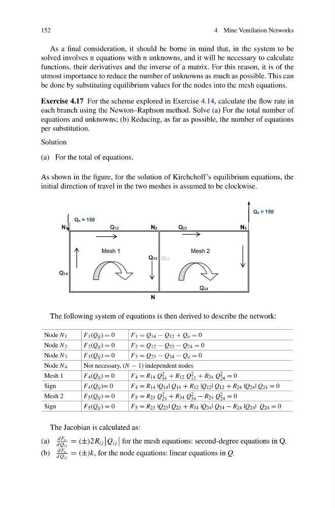
As shown in the figure, for the solution of Kirchchoff’s equilibrium equations, the
initial direction of travel in the two meshes is assumed to be clockwise.
Qa = 150
Qs = 150
N1
Q12
N2
Q23
N3
Mesh 1
Mesh 2
Q24 Q24
Q14
Q34
N
The following system of equations is then derived to describe the network:
Node N 1
F 1 (Q ij ) = 0
F 1 = Q 14 − Q 12 + Q a = 0
Node N 2
F 2 (Q ij ) = 0
F 2 = Q 12 − Q 23 − Q 24 = 0
Node N 3
F 3 (Q ij ) = 0
F 3 = Q 23 − Q 34 − Q a = 0
Node N 4
Not necessary, (N − 1) independent nodes
Mesh 1
F 4 (Q ij ) = 0
F 4 = R 14 Q 2
14 + R 12 Q 2
12 + R 24 Q 2
24 = 0
Sign
F 4 (Q ij )= 0
F 4 = R 14 |Q 14 | Q 14 + R 12 |Q 12 | Q 12 + R 24 |Q 24 | Q 24 = 0
Mesh 2
F 5 (Q ij ) = 0
F 5 = R 23 Q 2
23 + R 34 Q 2
34 − R 24 Q 2
24 = 0
Sign
F 5 (Q ij ) = 0
F 5 = R 23 |Q 23 | Q 23 + R 34 |Q 34 | Q 34 − R 24 |Q 24 | Q 24 = 0
The Jacobian is calculated as:
(a)
d F n
d Q i j
= (±)2R i j
Q i j
for the mesh equations: second-degree equations in Q.
(b)
d F n
d Q i j
= (±)k, for the node equations: linear equations in Q.
4 Mine Ventilation Networks
As a final consideration, it should be borne in mind that, in the system to be
solved involves n equations with n unknowns, and it will be necessary to calculate
functions, their derivatives and the inverse of a matrix. For this reason, it is of the
utmost importance to reduce the number of unknowns as much as possible. This can
be done by substituting equilibrium values for the nodes into the mesh equations.
Exercise 4.17 For the scheme explored in Exercise 4.14, calculate the flow rate in
each branch using the Newton–Raphson method. Solve (a) For the total number of
equations and unknowns; (b) Reducing, as far as possible, the number of equations
per substitution.
Solution
(a) For the total of equations.
As shown in the figure, for the solution of Kirchchoff’s equilibrium equations, the
initial direction of travel in the two meshes is assumed to be clockwise.
Qa = 150
Qs = 150
N1
Q12
N2
Q23
N3
Mesh 1
Mesh 2
Q24 Q24
Q14
Q34
N
The following system of equations is then derived to describe the network:
Node N 1
F 1 (Q ij ) = 0
F 1 = Q 14 − Q 12 + Q a = 0
Node N 2
F 2 (Q ij ) = 0
F 2 = Q 12 − Q 23 − Q 24 = 0
Node N 3
F 3 (Q ij ) = 0
F 3 = Q 23 − Q 34 − Q a = 0
Node N 4
Not necessary, (N − 1) independent nodes
Mesh 1
F 4 (Q ij ) = 0
F 4 = R 14 Q 2
14 + R 12 Q 2
12 + R 24 Q 2
24 = 0
Sign
F 4 (Q ij )= 0
F 4 = R 14 |Q 14 | Q 14 + R 12 |Q 12 | Q 12 + R 24 |Q 24 | Q 24 = 0
Mesh 2
F 5 (Q ij ) = 0
F 5 = R 23 Q 2
23 + R 34 Q 2
34 − R 24 Q 2
24 = 0
Sign
F 5 (Q ij ) = 0
F 5 = R 23 |Q 23 | Q 23 + R 34 |Q 34 | Q 34 − R 24 |Q 24 | Q 24 = 0
The Jacobian is calculated as:
(a)
d F n
d Q i j
= (±)2R i j
Q i j
for the mesh equations: second-degree equations in Q.
(b)
d F n
d Q i j
= (±)k, for the node equations: linear equations in Q.