

370
Shalabh and S. S. Dhar
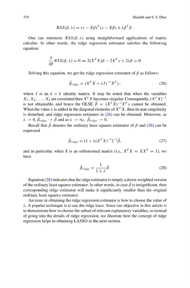
RSS(β, λ) = (y − Xβ)
T
(y − Xβ) + λβ
T
β .
One can minimize RSS(β, λ) using straightforward applications of matrix
calculus. In other words, the ridge regression estimator satisfies the following
equation:
∂
∂β
RSS(β, λ) = 0 ⇔ 2(X
T X )β − 2X
T y + 2λβ = 0.
Solving this equation, we get the ridge regression estimator of β as follows:
ˆ
β ridge = (X
T X + λI )
−1 X
T y,
(26)
where I is an k × k identity matrix. It may be noted that when the variables
X 1 , X 2 , . . . , X k are correlated then X
T X becomes singular. Consequently, (X
T X )
−1
is not obtainable, and hence the OLSE ˆ
β = (X
T X )
−1 X
T y cannot be obtained.
When the value λ is added in the diagonal elements of X
T X, then its non-singularity
is disturbed, and ridge regression estimator in (26) can be obtained. Moreover, as
λ → 0, ˆ
β ridge → ˆ
β and as λ → ∞, ˆ
β ridge → 0.
Recall that ˆ
β denotes the ordinary least squares estimator of β and (26) can be
expressed
ˆ
β ridge = [I + λ(X
T X )
−1
]
−1 ˆ
β,
(27)
and in particular, when X is an orthonormal matrix (i.e., X
T X = X X
T
= I ), we
have
ˆ
β ridge =
1
1 + λ
ˆ
β.
(28)
Equation (28) indicates that the ridge estimator is simply a down-weighted version
of the ordinary least squares estimator. In other words, in case ˆ
β is insignificant, then
corresponding ridge estimator will make it significantly smaller than the original
ordinary least squares estimator.
An issue in obtaining the ridge regression estimator is how to choose the value of
λ. A popular technique is to use the ridge trace. Since our objective in this article is
to demonstrate how to choose the subset of relevant explanatory variables, so instead
of going into the details of ridge regression, we illustrate how the concept of ridge
regression helps in obtaining LASSO in the next section.
Shalabh and S. S. Dhar
RSS(β, λ) = (y − Xβ)
T
(y − Xβ) + λβ
T
β .
One can minimize RSS(β, λ) using straightforward applications of matrix
calculus. In other words, the ridge regression estimator satisfies the following
equation:
∂
∂β
RSS(β, λ) = 0 ⇔ 2(X
T X )β − 2X
T y + 2λβ = 0.
Solving this equation, we get the ridge regression estimator of β as follows:
ˆ
β ridge = (X
T X + λI )
−1 X
T y,
(26)
where I is an k × k identity matrix. It may be noted that when the variables
X 1 , X 2 , . . . , X k are correlated then X
T X becomes singular. Consequently, (X
T X )
−1
is not obtainable, and hence the OLSE ˆ
β = (X
T X )
−1 X
T y cannot be obtained.
When the value λ is added in the diagonal elements of X
T X, then its non-singularity
is disturbed, and ridge regression estimator in (26) can be obtained. Moreover, as
λ → 0, ˆ
β ridge → ˆ
β and as λ → ∞, ˆ
β ridge → 0.
Recall that ˆ
β denotes the ordinary least squares estimator of β and (26) can be
expressed
ˆ
β ridge = [I + λ(X
T X )
−1
]
−1 ˆ
β,
(27)
and in particular, when X is an orthonormal matrix (i.e., X
T X = X X
T
= I ), we
have
ˆ
β ridge =
1
1 + λ
ˆ
β.
(28)
Equation (28) indicates that the ridge estimator is simply a down-weighted version
of the ordinary least squares estimator. In other words, in case ˆ
β is insignificant, then
corresponding ridge estimator will make it significantly smaller than the original
ordinary least squares estimator.
An issue in obtaining the ridge regression estimator is how to choose the value of
λ. A popular technique is to use the ridge trace. Since our objective in this article is
to demonstrate how to choose the subset of relevant explanatory variables, so instead
of going into the details of ridge regression, we illustrate how the concept of ridge
regression helps in obtaining LASSO in the next section.