

7.7 Mathematical Model of Three-Layer Micro- and Nano-Beams
273
7.7.3 Equations of Motion and Boundary Conditions for the
Three-Layer Beam
The state/motion equations as well as the associated boundary conditions corresponding to the assumed kinematic hypotheses are yielded directly from Hamilton’s
principle
δ
t 2
t 1
(T − U + W ) d t = 0,
(7.135)
where U is the energy of deformation of the bended isotropic three-layer linear elastic beam, T is its kinetic energy, whereas W presents the work of external forces.
Therefore, we study the three-layer beam of length L subjected to both external
transversal load q (x) and external stresses: normal bσ and tangential bτ with intensities on boundaries
σ 0 , τ 0 | x=0 ,
σ L , τ L | x=L .
(7.136)
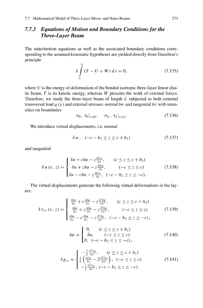
We introduce virtual displacements, i.e. normal
δ w , (−c − h 2 ≤ z ≤ c + h 1 )
(7.137)
and tangential
δ u (x, z) =
⎧
⎪ ⎨
⎪ ⎩
δu + cδα − z
∂δ w
∂ x
,
(c ≤ z ≤ c + h 1 )
δu + zδα − z
∂δ w
∂ x
,
(−c ≤ z ≤ c)
δu − cδα − z
∂δ w
∂ x
, (−c − h 2 ≤ z ≤ −c) .
(7.138)
The virtual displacements generate the following virtual deformations in the layers:
δ ε xx (x, z) =
⎧
⎪ ⎪ ⎨
⎪ ⎪ ⎩
∂δu
∂ x
+ c
∂δα
∂ x
− z
∂
2 δw
∂ x 2 ,
(c ≤ z ≤ c + h 1 )
∂δu
∂ x
+ z
∂δα
∂ x
− z
∂
2 δw
∂ x 2 ,
(−c ≤ z ≤ c)
∂δu
∂ x
− c
∂δα
∂ x
− z
∂
2 δw
∂ x 2 , (−c − h 2 ≤ z ≤ −c) ,
(7.139)
δα =
⎧
⎨
⎩
0,
(c ≤ z ≤ c + h 1 )
δα,
(−c ≤ z ≤ c)
0, (−c − h 2 ≤ z ≤ −c) ,
(7.140)
δχ xy =
⎧
⎪ ⎨
⎪ ⎩
−
1
2
∂
2 δ w
∂ x 2 ,
(c ≤ z ≤ c + h 1 )
1
4
∂δ α
∂ x
− 2
∂
2 δ w
∂ x 2
, (−c ≤ z ≤ c)
−
1
2
∂
2 δ w
∂ x 2 , (−c − h 2 ≤ z ≤ −c) .
(7.141)
273
7.7.3 Equations of Motion and Boundary Conditions for the
Three-Layer Beam
The state/motion equations as well as the associated boundary conditions corresponding to the assumed kinematic hypotheses are yielded directly from Hamilton’s
principle
δ
t 2
t 1
(T − U + W ) d t = 0,
(7.135)
where U is the energy of deformation of the bended isotropic three-layer linear elastic beam, T is its kinetic energy, whereas W presents the work of external forces.
Therefore, we study the three-layer beam of length L subjected to both external
transversal load q (x) and external stresses: normal bσ and tangential bτ with intensities on boundaries
σ 0 , τ 0 | x=0 ,
σ L , τ L | x=L .
(7.136)
We introduce virtual displacements, i.e. normal
δ w , (−c − h 2 ≤ z ≤ c + h 1 )
(7.137)
and tangential
δ u (x, z) =
⎧
⎪ ⎨
⎪ ⎩
δu + cδα − z
∂δ w
∂ x
,
(c ≤ z ≤ c + h 1 )
δu + zδα − z
∂δ w
∂ x
,
(−c ≤ z ≤ c)
δu − cδα − z
∂δ w
∂ x
, (−c − h 2 ≤ z ≤ −c) .
(7.138)
The virtual displacements generate the following virtual deformations in the layers:
δ ε xx (x, z) =
⎧
⎪ ⎪ ⎨
⎪ ⎪ ⎩
∂δu
∂ x
+ c
∂δα
∂ x
− z
∂
2 δw
∂ x 2 ,
(c ≤ z ≤ c + h 1 )
∂δu
∂ x
+ z
∂δα
∂ x
− z
∂
2 δw
∂ x 2 ,
(−c ≤ z ≤ c)
∂δu
∂ x
− c
∂δα
∂ x
− z
∂
2 δw
∂ x 2 , (−c − h 2 ≤ z ≤ −c) ,
(7.139)
δα =
⎧
⎨
⎩
0,
(c ≤ z ≤ c + h 1 )
δα,
(−c ≤ z ≤ c)
0, (−c − h 2 ≤ z ≤ −c) ,
(7.140)
δχ xy =
⎧
⎪ ⎨
⎪ ⎩
−
1
2
∂
2 δ w
∂ x 2 ,
(c ≤ z ≤ c + h 1 )
1
4
∂δ α
∂ x
− 2
∂
2 δ w
∂ x 2
, (−c ≤ z ≤ c)
−
1
2
∂
2 δ w
∂ x 2 , (−c − h 2 ≤ z ≤ −c) .
(7.141)