

244
7 Mathematical Models of Functionally Graded Beams in Temperature Field
-5
-4
-3
-2
-1
0 q
600
400
200
0
w
3
1
2
-5
-4
-3
-2
-1
0 q
400
200
0
w
6
4
5
-5
-4
-3
-2
-1
0 q
600
300
0
w
7
4
1
450
150
8
a)
b)
c)
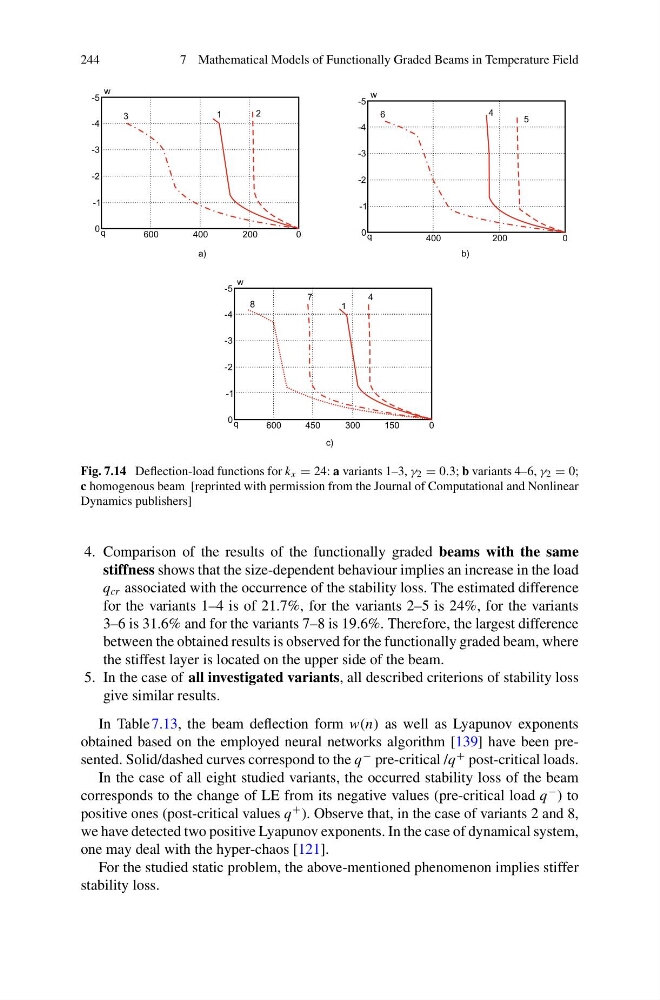
Fig. 7.14 Deflection-load functions for k x = 24: a variants 1–3, γ 2 = 0.3; b variants 4–6, γ 2 = 0;
c homogenous beam [reprinted with permission from the Journal of Computational and Nonlinear
Dynamics publishers]
4. Comparison of the results of the functionally graded beams with the same
stiffness shows that the size-dependent behaviour implies an increase in the load
q cr associated with the occurrence of the stability loss. The estimated difference
for the variants 1–4 is of 21.7%, for the variants 2–5 is 24%, for the variants
3–6 is 31.6% and for the variants 7–8 is 19.6%. Therefore, the largest difference
between the obtained results is observed for the functionally graded beam, where
the stiffest layer is located on the upper side of the beam.
5. In the case of all investigated variants, all described criterions of stability loss
give similar results.
In Table 7.13, the beam deflection form w(n) as well as Lyapunov exponents
obtained based on the employed neural networks algorithm [139] have been presented. Solid/dashed curves correspond to the q
− pre-critical /q
+ post-critical loads.
In the case of all eight studied variants, the occurred stability loss of the beam
corresponds to the change of LE from its negative values (pre-critical load q
− ) to
positive ones (post-critical values q
+ ). Observe that, in the case of variants 2 and 8,
we have detected two positive Lyapunov exponents. In the case of dynamical system,
one may deal with the hyper-chaos [121].
For the studied static problem, the above-mentioned phenomenon implies stiffer
stability loss.
7 Mathematical Models of Functionally Graded Beams in Temperature Field
-5
-4
-3
-2
-1
0 q
600
400
200
0
w
3
1
2
-5
-4
-3
-2
-1
0 q
400
200
0
w
6
4
5
-5
-4
-3
-2
-1
0 q
600
300
0
w
7
4
1
450
150
8
a)
b)
c)
Fig. 7.14 Deflection-load functions for k x = 24: a variants 1–3, γ 2 = 0.3; b variants 4–6, γ 2 = 0;
c homogenous beam [reprinted with permission from the Journal of Computational and Nonlinear
Dynamics publishers]
4. Comparison of the results of the functionally graded beams with the same
stiffness shows that the size-dependent behaviour implies an increase in the load
q cr associated with the occurrence of the stability loss. The estimated difference
for the variants 1–4 is of 21.7%, for the variants 2–5 is 24%, for the variants
3–6 is 31.6% and for the variants 7–8 is 19.6%. Therefore, the largest difference
between the obtained results is observed for the functionally graded beam, where
the stiffest layer is located on the upper side of the beam.
5. In the case of all investigated variants, all described criterions of stability loss
give similar results.
In Table 7.13, the beam deflection form w(n) as well as Lyapunov exponents
obtained based on the employed neural networks algorithm [139] have been presented. Solid/dashed curves correspond to the q
− pre-critical /q
+ post-critical loads.
In the case of all eight studied variants, the occurred stability loss of the beam
corresponds to the change of LE from its negative values (pre-critical load q
− ) to
positive ones (post-critical values q
+ ). Observe that, in the case of variants 2 and 8,
we have detected two positive Lyapunov exponents. In the case of dynamical system,
one may deal with the hyper-chaos [121].
For the studied static problem, the above-mentioned phenomenon implies stiffer
stability loss.