

172
6 Mathematical Models of Micro- and Nano-cylindrical Panels in Temperature Field
6.6.1 Analysis of Dynamic Characteristics of the
Bernoulli–Euler, Timoshenko and Sheremetev–Pelekh
Models for the Size-Dependent Beams Versus the Size
Length
In this subsection, we report a comparison of the dynamic problems of beams subject
to the transversal load q = q 0 sin(ω p t) for the fixed value of the length scale material
parameter l/ h = 0.3. The following load parameters are taken: q 0 = 4000, ω p = 9.
The frequency ω p = 9 is chosen to avoid possible resonances, i.e. if differs from the
beam natural frequencies.
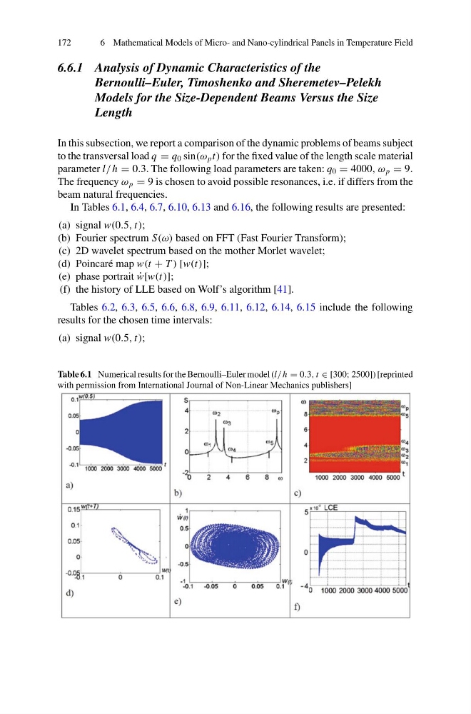
In Tables 6.1, 6.4, 6.7, 6.10, 6.13 and 6.16, the following results are presented:
(a) signal w(0.5, t);
(b) Fourier spectrum S(ω) based on FFT (Fast Fourier Transform);
(c) 2D wavelet spectrum based on the mother Morlet wavelet;
(d) Poincaré map w(t + T ) [w(t)];
(e) phase portrait ˙
w[w(t)];
(f) the history of LLE based on Wolf’s algorithm [41].
Tables 6.2, 6.3, 6.5, 6.6, 6.8, 6.9, 6.11, 6.12, 6.14, 6.15 include the following
results for the chosen time intervals:
(a) signal w(0.5, t);
Table 6.1 Numerical results for the Bernoulli–Euler model (l/ h = 0.3, t ∈ [300; 2500]) [reprinted
with permission from International Journal of Non-Linear Mechanics publishers]
6 Mathematical Models of Micro- and Nano-cylindrical Panels in Temperature Field
6.6.1 Analysis of Dynamic Characteristics of the
Bernoulli–Euler, Timoshenko and Sheremetev–Pelekh
Models for the Size-Dependent Beams Versus the Size
Length
In this subsection, we report a comparison of the dynamic problems of beams subject
to the transversal load q = q 0 sin(ω p t) for the fixed value of the length scale material
parameter l/ h = 0.3. The following load parameters are taken: q 0 = 4000, ω p = 9.
The frequency ω p = 9 is chosen to avoid possible resonances, i.e. if differs from the
beam natural frequencies.
In Tables 6.1, 6.4, 6.7, 6.10, 6.13 and 6.16, the following results are presented:
(a) signal w(0.5, t);
(b) Fourier spectrum S(ω) based on FFT (Fast Fourier Transform);
(c) 2D wavelet spectrum based on the mother Morlet wavelet;
(d) Poincaré map w(t + T ) [w(t)];
(e) phase portrait ˙
w[w(t)];
(f) the history of LLE based on Wolf’s algorithm [41].
Tables 6.2, 6.3, 6.5, 6.6, 6.8, 6.9, 6.11, 6.12, 6.14, 6.15 include the following
results for the chosen time intervals:
(a) signal w(0.5, t);
Table 6.1 Numerical results for the Bernoulli–Euler model (l/ h = 0.3, t ∈ [300; 2500]) [reprinted
with permission from International Journal of Non-Linear Mechanics publishers]