

6.4 Technical Theory for the Different Models
161
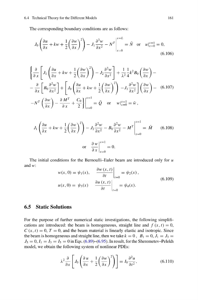
The corresponding boundary conditions are as follows:
J 0
∂u
∂ x
+ kw +
1
2
∂w
∂ x
2
− J 1
∂
2 w
∂ x 2 − N
T
x=L
x=0
= ¯
N or u|
x=1
x=0 = 0,
(6.106)
∂
∂ x
J 1
∂u
∂ x
+ kw +
1
2
∂w
∂ x
2
− J 2
∂
2 w
∂ x 2
+
1
λ 2
1
4
k
2 B 0
∂w
∂ x
−
−
∂
∂ x
B 0
∂
2 w
∂ x 2
+
J 0
∂u
∂ x
+ kw +
1
2
∂w
∂ x
2
−J 1
∂
2 w
∂ x 2
∂w
∂ x
−
−N
T
∂w
∂ x
−
∂ M
T
∂ x
+
C 0
2
x=1
x=0
= ¯
Q or w|
x=1
x=0 = ¯
w ,
(6.107)
J 1
∂u
∂ x
+ kw +
1
2
∂w
∂ x
2
− J 2
∂
2 w
∂ x 2 − B 0
∂
2 w
∂ x 2 − M
T
x=1
x=0
= ¯
M
(6.108)
or
∂ w
∂ x
x=1
x=0
= 0.
The initial conditions for the Bernoulli–Euler beam are introduced only for u
and w:
w(x, 0) = ψ 1 (x),
∂w (x, t)
∂t
t=0
= ψ 2 (x) ,
u(x, 0) = ψ 3 (x)
∂u (x, t)
∂t
t=0
= ψ 4 (x).
(6.109)
6.5 Static Solutions
For the purpose of further numerical static investigations, the following simplifications are introduced: the beam is homogeneous, straight line and f (x, t) = 0,
C (x, t) = 0, T = 0, and the beam material is linearly elastic and isotropic. Since
the beam is homogeneous and straight line, then we take k = 0 , B 1 = 0, J 1 = J 3 =
J 5 = 0, I 1 = I 3 = I 5 = 0 in Eqs. (6.89)–(6.95). In result, for the Sheremetev–Pelekh
model, we obtain the following system of nonlinear PDEs:
λ
2 ∂
∂ x
J 0
∂ u
∂ x
+
1
2
∂w
∂ x
2
= I 0
∂
2 u
∂t 2 ,
(6.110)
161
The corresponding boundary conditions are as follows:
J 0
∂u
∂ x
+ kw +
1
2
∂w
∂ x
2
− J 1
∂
2 w
∂ x 2 − N
T
x=L
x=0
= ¯
N or u|
x=1
x=0 = 0,
(6.106)
∂
∂ x
J 1
∂u
∂ x
+ kw +
1
2
∂w
∂ x
2
− J 2
∂
2 w
∂ x 2
+
1
λ 2
1
4
k
2 B 0
∂w
∂ x
−
−
∂
∂ x
B 0
∂
2 w
∂ x 2
+
J 0
∂u
∂ x
+ kw +
1
2
∂w
∂ x
2
−J 1
∂
2 w
∂ x 2
∂w
∂ x
−
−N
T
∂w
∂ x
−
∂ M
T
∂ x
+
C 0
2
x=1
x=0
= ¯
Q or w|
x=1
x=0 = ¯
w ,
(6.107)
J 1
∂u
∂ x
+ kw +
1
2
∂w
∂ x
2
− J 2
∂
2 w
∂ x 2 − B 0
∂
2 w
∂ x 2 − M
T
x=1
x=0
= ¯
M
(6.108)
or
∂ w
∂ x
x=1
x=0
= 0.
The initial conditions for the Bernoulli–Euler beam are introduced only for u
and w:
w(x, 0) = ψ 1 (x),
∂w (x, t)
∂t
t=0
= ψ 2 (x) ,
u(x, 0) = ψ 3 (x)
∂u (x, t)
∂t
t=0
= ψ 4 (x).
(6.109)
6.5 Static Solutions
For the purpose of further numerical static investigations, the following simplifications are introduced: the beam is homogeneous, straight line and f (x, t) = 0,
C (x, t) = 0, T = 0, and the beam material is linearly elastic and isotropic. Since
the beam is homogeneous and straight line, then we take k = 0 , B 1 = 0, J 1 = J 3 =
J 5 = 0, I 1 = I 3 = I 5 = 0 in Eqs. (6.89)–(6.95). In result, for the Sheremetev–Pelekh
model, we obtain the following system of nonlinear PDEs:
λ
2 ∂
∂ x
J 0
∂ u
∂ x
+
1
2
∂w
∂ x
2
= I 0
∂
2 u
∂t 2 ,
(6.110)