

6.4 Technical Theory for the Different Models
159
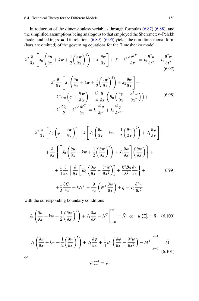
Introduction of the dimensionless variables through formulas (6.87) (6.88), and
the simplified assumptions being analogous to that employed the Sheremetev–Pelekh
model and taking α = 0 in relations (6.89)–(6.95) yields the non-dimensional form
(bars are omitted) of the governing equations for the Timoshenko model:
λ
2 ∂
∂ x
J 0
∂u
∂ x
+ kw +
1
2
∂w
∂ x
2
+ J 1
∂ϕ
∂ x
+ f − λ
2 ∂ N
T
∂ x
= I 0
∂
2 u
∂t 2 + I 1
∂
2
ϕ
∂t 2 ,
(6.97)
λ
2 ∂
∂ x
J 1
∂u
∂ x
+ kw +
1
2
∂w
∂ x
2
+ J 2
∂ϕ
∂ x
−
− λ
4 A 0
ϕ +
∂ w
∂ x
+
λ
2
4
∂
∂ x
B 0
∂ϕ
∂ x
−
∂
2 w
∂ x 2
+
+ λ
2 C 0
2
− λ
2 ∂ M
T
∂ x
= I 1
∂
2 u
∂t 2 + I 2
∂
2
ϕ
∂t 2 ,
(6.98)
λ
2 ∂
∂ x
A 0
ϕ +
∂w
∂ x
− k
J 0
∂u
∂ x
+ kw +
1
2
∂w
∂ x
2
+ J 1
∂ϕ
∂ x
+
+
∂
∂ x
J 0
∂u
∂ x
+ kw +
1
2
∂w
∂ x
2
+ J 1
∂ϕ
∂ x
∂w
∂ x
+
+
1
4
∂
∂ x
∂
∂ x
B 0
∂ϕ
∂ x
−
∂
2 w
∂ x 2
+
k
2 B 0
λ 2
∂w
∂ x
+
(6.99)
+
1
2
∂C 0
∂ x
+ k N
T
−
∂
∂ x
N
T ∂w
∂ x
+ q = I 0
∂
2 w
∂t 2
with the corresponding boundary conditions
J 0
∂u
∂ x
+ kw +
1
2
∂w
∂ x
2
+ J 1
∂ϕ
∂ x
− N
T
x=1
x=0
= ¯
N or u|
x=1
x=0 = ¯
u, (6.100)
J 1
∂u
∂ x
+ kw +
1
2
∂w
∂ x
2
+ J 2
∂ϕ
∂ x
+
1
4
B 0
∂ϕ
∂ x
−
∂
2 w
∂ x 2
− M
T
x=1
x=0
= ¯
M
(6.101)
or
ϕ|
x=1
x=0 = ¯
ϕ,
159
Introduction of the dimensionless variables through formulas (6.87) (6.88), and
the simplified assumptions being analogous to that employed the Sheremetev–Pelekh
model and taking α = 0 in relations (6.89)–(6.95) yields the non-dimensional form
(bars are omitted) of the governing equations for the Timoshenko model:
λ
2 ∂
∂ x
J 0
∂u
∂ x
+ kw +
1
2
∂w
∂ x
2
+ J 1
∂ϕ
∂ x
+ f − λ
2 ∂ N
T
∂ x
= I 0
∂
2 u
∂t 2 + I 1
∂
2
ϕ
∂t 2 ,
(6.97)
λ
2 ∂
∂ x
J 1
∂u
∂ x
+ kw +
1
2
∂w
∂ x
2
+ J 2
∂ϕ
∂ x
−
− λ
4 A 0
ϕ +
∂ w
∂ x
+
λ
2
4
∂
∂ x
B 0
∂ϕ
∂ x
−
∂
2 w
∂ x 2
+
+ λ
2 C 0
2
− λ
2 ∂ M
T
∂ x
= I 1
∂
2 u
∂t 2 + I 2
∂
2
ϕ
∂t 2 ,
(6.98)
λ
2 ∂
∂ x
A 0
ϕ +
∂w
∂ x
− k
J 0
∂u
∂ x
+ kw +
1
2
∂w
∂ x
2
+ J 1
∂ϕ
∂ x
+
+
∂
∂ x
J 0
∂u
∂ x
+ kw +
1
2
∂w
∂ x
2
+ J 1
∂ϕ
∂ x
∂w
∂ x
+
+
1
4
∂
∂ x
∂
∂ x
B 0
∂ϕ
∂ x
−
∂
2 w
∂ x 2
+
k
2 B 0
λ 2
∂w
∂ x
+
(6.99)
+
1
2
∂C 0
∂ x
+ k N
T
−
∂
∂ x
N
T ∂w
∂ x
+ q = I 0
∂
2 w
∂t 2
with the corresponding boundary conditions
J 0
∂u
∂ x
+ kw +
1
2
∂w
∂ x
2
+ J 1
∂ϕ
∂ x
− N
T
x=1
x=0
= ¯
N or u|
x=1
x=0 = ¯
u, (6.100)
J 1
∂u
∂ x
+ kw +
1
2
∂w
∂ x
2
+ J 2
∂ϕ
∂ x
+
1
4
B 0
∂ϕ
∂ x
−
∂
2 w
∂ x 2
− M
T
x=1
x=0
= ¯
M
(6.101)
or
ϕ|
x=1
x=0 = ¯
ϕ,