

6.4 Technical Theory for the Different Models
151
− N
T
∂w
∂ x
− α
∂ P
T
∂ x
x=L
x=0
= ¯
Q or w|
x=L
x=0 = ¯
w
α
J 3
∂u
∂ x
+ kw +
1
2
∂w
∂ x
2
+ (J 4 − α J 6 )
∂ϕ
∂ x
− α J 6
∂
2 w
∂ x 2
+
+
1
2
B 0
∂ϕ
∂ x
−
∂
2 w
∂ x 2
− 3α B 2
∂ϕ
∂ x
+
∂
2 w
∂ x 2
+
(6.74)
+
3α
4
B 2
∂ϕ
∂ x
−
∂
2 w
∂ x 2
− 3α B 4
∂ϕ
∂ x
+
∂
2 w
∂ x 2
− α P
T
x=L
x=0
= α ¯
P
or
∂w
∂ x
x=L
x=0
=
____
∂w
∂ x
.
Equations of Motion for the Timoshenko and Bernoulli–Euler Models
The second approximation model proposed by Timoshenko [49] does not take into
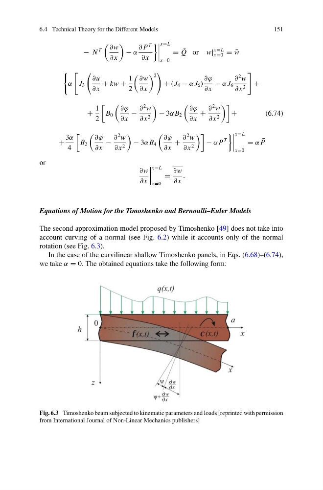
account curving of a normal (see Fig. 6.2) while it accounts only of the normal
rotation (see Fig. 6.3).
In the case of the curvilinear shallow Timoshenko panels, in Eqs. (6.68)–(6.74),
we take α = 0. The obtained equations take the following form:
Fig. 6.3 Timoshenko beam subjected to kinematic parameters and loads [reprinted with permission
from International Journal of Non-Linear Mechanics publishers]
151
− N
T
∂w
∂ x
− α
∂ P
T
∂ x
x=L
x=0
= ¯
Q or w|
x=L
x=0 = ¯
w
α
J 3
∂u
∂ x
+ kw +
1
2
∂w
∂ x
2
+ (J 4 − α J 6 )
∂ϕ
∂ x
− α J 6
∂
2 w
∂ x 2
+
+
1
2
B 0
∂ϕ
∂ x
−
∂
2 w
∂ x 2
− 3α B 2
∂ϕ
∂ x
+
∂
2 w
∂ x 2
+
(6.74)
+
3α
4
B 2
∂ϕ
∂ x
−
∂
2 w
∂ x 2
− 3α B 4
∂ϕ
∂ x
+
∂
2 w
∂ x 2
− α P
T
x=L
x=0
= α ¯
P
or
∂w
∂ x
x=L
x=0
=
____
∂w
∂ x
.
Equations of Motion for the Timoshenko and Bernoulli–Euler Models
The second approximation model proposed by Timoshenko [49] does not take into
account curving of a normal (see Fig. 6.2) while it accounts only of the normal
rotation (see Fig. 6.3).
In the case of the curvilinear shallow Timoshenko panels, in Eqs. (6.68)–(6.74),
we take α = 0. The obtained equations take the following form:
Fig. 6.3 Timoshenko beam subjected to kinematic parameters and loads [reprinted with permission
from International Journal of Non-Linear Mechanics publishers]