

6.4 Technical Theory for the Different Models
147
6.4 Technical Theory for the Sheremetev–Pelekh,
Timoshenko and Bernoulli–Euler Models
The structure of equations (6.40)–(6.42) of the general theory of curvilinear panels
is rather complex, and hence getting a reliable solution to those equations for a series
of problems requires to overcome of serious mathematical difficulties. Therefore,
there is a need to simplify those fundamental equations and choose their variants
being suitable for account of features of the most important problems that occurred
in practice. On a basis of numerous theoretical investigations [45, 47, 48], it has been
shown that in majority of the engineering problems it is sufficient to consider the
middle panel surface as shallow one. In the following, we will present the simplified
variant of the fundamental governing equations of theory of curvilinear panels being
based on that shallowly panel hypothesis. Recall that a panel or a beam is defined as
shallow if owing to the Vlasov statement kh ≤ 1/30. The theory with the introduced
assumptions will be further called technical theory of curvilinear panels.
Besides the fundamental hypothesis, the so far introduced technical theory
employs the following hypotheses in the geometric relations (6.8), and the deformations caused by tangential displacement u
z can be neglected, i.e. we take β = 0;
the curvilinear coordinate ϑ is chosen to satisfy the inequality kh << 1. Validation
of the latter assumption into theory of shell has been carried out by Mushtari [47, 48].
He showed that neglection of the tangential displacements will be more strongly realized by decreasing stresses caused by moments in comparison to stresses originated
from forces.
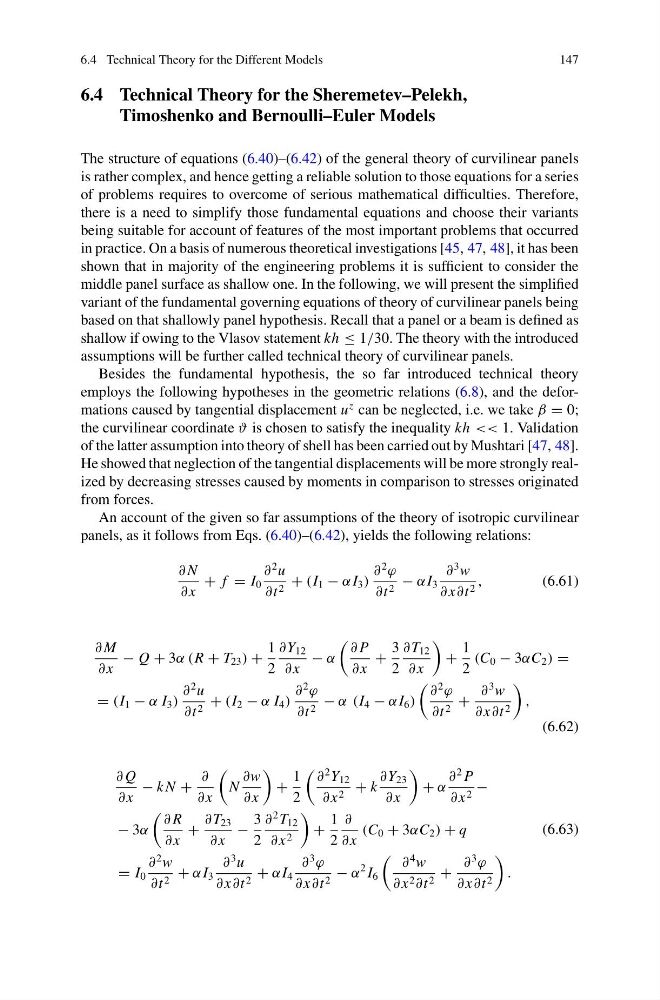
An account of the given so far assumptions of the theory of isotropic curvilinear
panels, as it follows from Eqs. (6.40)–(6.42), yields the following relations:
∂ N
∂ x
+ f = I 0
∂
2 u
∂t 2 + (I 1 − α I 3 )
∂
2
ϕ
∂t 2 − α I 3
∂
3 w
∂ x∂t 2 ,
(6.61)
∂ M
∂ x
− Q + 3α (R + T 23 ) +
1
2
∂Y 12
∂ x
− α
∂ P
∂ x
+
3
2
∂ T 12
∂ x
+
1
2
(C 0 − 3αC 2 ) =
= (I 1 − α I 3 )
∂
2 u
∂t 2 + (I 2 − α I 4 )
∂
2
ϕ
∂t 2 − α (I 4 − α I 6 )
∂
2
ϕ
∂t 2 +
∂
3 w
∂ x∂t 2
,
(6.62)
∂ Q
∂ x
− k N +
∂
∂ x
N
∂w
∂ x
+
1
2
∂
2 Y 12
∂ x 2 + k
∂Y 23
∂ x
+ α
∂
2 P
∂ x 2 −
− 3α
∂ R
∂ x
+
∂ T 23
∂ x
−
3
2
∂
2 T 12
∂ x 2
+
1
2
∂
∂ x
(C 0 + 3αC 2 ) + q
= I 0
∂
2 w
∂t 2 + α I 3
∂
3 u
∂ x∂t 2 + α I 4
∂
3
ϕ
∂ x∂t 2 − α
2 I 6
∂
4 w
∂ x 2 ∂t 2 +
∂
3
ϕ
∂ x∂t 2
.
(6.63)
147
6.4 Technical Theory for the Sheremetev–Pelekh,
Timoshenko and Bernoulli–Euler Models
The structure of equations (6.40)–(6.42) of the general theory of curvilinear panels
is rather complex, and hence getting a reliable solution to those equations for a series
of problems requires to overcome of serious mathematical difficulties. Therefore,
there is a need to simplify those fundamental equations and choose their variants
being suitable for account of features of the most important problems that occurred
in practice. On a basis of numerous theoretical investigations [45, 47, 48], it has been
shown that in majority of the engineering problems it is sufficient to consider the
middle panel surface as shallow one. In the following, we will present the simplified
variant of the fundamental governing equations of theory of curvilinear panels being
based on that shallowly panel hypothesis. Recall that a panel or a beam is defined as
shallow if owing to the Vlasov statement kh ≤ 1/30. The theory with the introduced
assumptions will be further called technical theory of curvilinear panels.
Besides the fundamental hypothesis, the so far introduced technical theory
employs the following hypotheses in the geometric relations (6.8), and the deformations caused by tangential displacement u
z can be neglected, i.e. we take β = 0;
the curvilinear coordinate ϑ is chosen to satisfy the inequality kh << 1. Validation
of the latter assumption into theory of shell has been carried out by Mushtari [47, 48].
He showed that neglection of the tangential displacements will be more strongly realized by decreasing stresses caused by moments in comparison to stresses originated
from forces.
An account of the given so far assumptions of the theory of isotropic curvilinear
panels, as it follows from Eqs. (6.40)–(6.42), yields the following relations:
∂ N
∂ x
+ f = I 0
∂
2 u
∂t 2 + (I 1 − α I 3 )
∂
2
ϕ
∂t 2 − α I 3
∂
3 w
∂ x∂t 2 ,
(6.61)
∂ M
∂ x
− Q + 3α (R + T 23 ) +
1
2
∂Y 12
∂ x
− α
∂ P
∂ x
+
3
2
∂ T 12
∂ x
+
1
2
(C 0 − 3αC 2 ) =
= (I 1 − α I 3 )
∂
2 u
∂t 2 + (I 2 − α I 4 )
∂
2
ϕ
∂t 2 − α (I 4 − α I 6 )
∂
2
ϕ
∂t 2 +
∂
3 w
∂ x∂t 2
,
(6.62)
∂ Q
∂ x
− k N +
∂
∂ x
N
∂w
∂ x
+
1
2
∂
2 Y 12
∂ x 2 + k
∂Y 23
∂ x
+ α
∂
2 P
∂ x 2 −
− 3α
∂ R
∂ x
+
∂ T 23
∂ x
−
3
2
∂
2 T 12
∂ x 2
+
1
2
∂
∂ x
(C 0 + 3αC 2 ) + q
= I 0
∂
2 w
∂t 2 + α I 3
∂
3 u
∂ x∂t 2 + α I 4
∂
3
ϕ
∂ x∂t 2 − α
2 I 6
∂
4 w
∂ x 2 ∂t 2 +
∂
3
ϕ
∂ x∂t 2
.
(6.63)