

5.5 Hyperchaotic Generalized Hénon Map
119
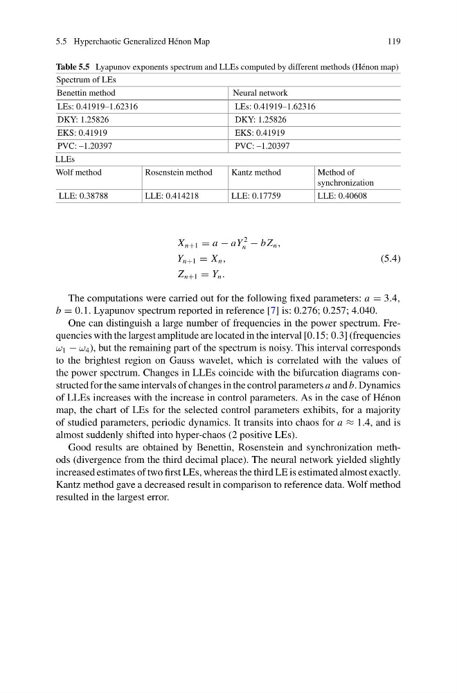
Table 5.5 Lyapunov exponents spectrum and LLEs computed by different methods (Hénon map)
Spectrum of LEs
Benettin method
Neural network
LEs: 0.41919–1.62316
LEs: 0.41919–1.62316
DKY: 1.25826
DKY: 1.25826
EKS: 0.41919
EKS: 0.41919
PVC: –1.20397
PVC: –1.20397
LLEs
Wolf method
Rosenstein method
Kantz method
Method of
synchronization
LLE: 0.38788
LLE: 0.414218
LLE: 0.17759
LLE: 0.40608
X n+1 = a − aY
2
n − bZ n ,
Y n+1 = X n ,
Z n+1 = Y n .
(5.4)
The computations were carried out for the following fixed parameters: a = 3.4,
b = 0.1. Lyapunov spectrum reported in reference [7] is: 0.276; 0.257; 4.040.
One can distinguish a large number of frequencies in the power spectrum. Frequencies with the largest amplitude are located in the interval [0.15; 0.3] (frequencies
ω 1 − ω 4 ), but the remaining part of the spectrum is noisy. This interval corresponds
to the brightest region on Gauss wavelet, which is correlated with the values of
the power spectrum. Changes in LLEs coincide with the bifurcation diagrams constructed for the same intervals of changes in the control parameters a and b. Dynamics
of LLEs increases with the increase in control parameters. As in the case of Hénon
map, the chart of LEs for the selected control parameters exhibits, for a majority
of studied parameters, periodic dynamics. It transits into chaos for a ≈ 1.4, and is
almost suddenly shifted into hyper-chaos (2 positive LEs).
Good results are obtained by Benettin, Rosenstein and synchronization methods (divergence from the third decimal place). The neural network yielded slightly
increased estimates of two first LEs, whereas the third LE is estimated almost exactly.
Kantz method gave a decreased result in comparison to reference data. Wolf method
resulted in the largest error.
119
Table 5.5 Lyapunov exponents spectrum and LLEs computed by different methods (Hénon map)
Spectrum of LEs
Benettin method
Neural network
LEs: 0.41919–1.62316
LEs: 0.41919–1.62316
DKY: 1.25826
DKY: 1.25826
EKS: 0.41919
EKS: 0.41919
PVC: –1.20397
PVC: –1.20397
LLEs
Wolf method
Rosenstein method
Kantz method
Method of
synchronization
LLE: 0.38788
LLE: 0.414218
LLE: 0.17759
LLE: 0.40608
X n+1 = a − aY
2
n − bZ n ,
Y n+1 = X n ,
Z n+1 = Y n .
(5.4)
The computations were carried out for the following fixed parameters: a = 3.4,
b = 0.1. Lyapunov spectrum reported in reference [7] is: 0.276; 0.257; 4.040.
One can distinguish a large number of frequencies in the power spectrum. Frequencies with the largest amplitude are located in the interval [0.15; 0.3] (frequencies
ω 1 − ω 4 ), but the remaining part of the spectrum is noisy. This interval corresponds
to the brightest region on Gauss wavelet, which is correlated with the values of
the power spectrum. Changes in LLEs coincide with the bifurcation diagrams constructed for the same intervals of changes in the control parameters a and b. Dynamics
of LLEs increases with the increase in control parameters. As in the case of Hénon
map, the chart of LEs for the selected control parameters exhibits, for a majority
of studied parameters, periodic dynamics. It transits into chaos for a ≈ 1.4, and is
almost suddenly shifted into hyper-chaos (2 positive LEs).
Good results are obtained by Benettin, Rosenstein and synchronization methods (divergence from the third decimal place). The neural network yielded slightly
increased estimates of two first LEs, whereas the third LE is estimated almost exactly.
Kantz method gave a decreased result in comparison to reference data. Wolf method
resulted in the largest error.