

3.9 Modification of the Neural Network Method
89
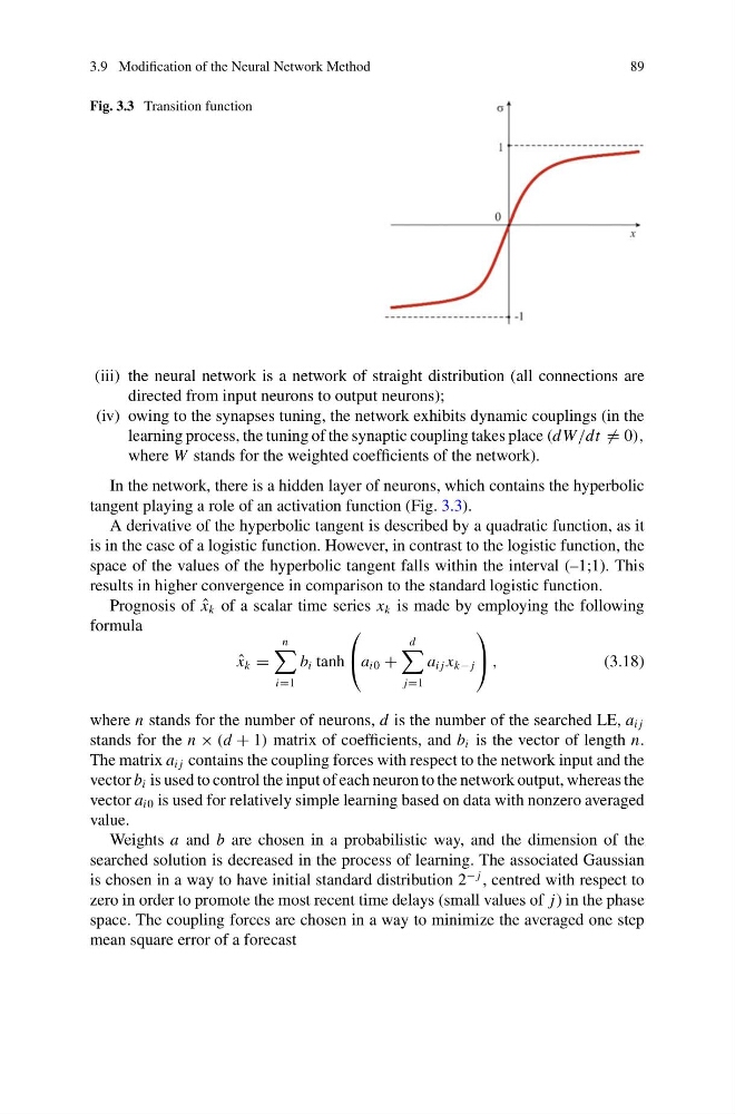
Fig. 3.3 Transition function
(iii) the neural network is a network of straight distribution (all connections are
directed from input neurons to output neurons);
(iv) owing to the synapses tuning, the network exhibits dynamic couplings (in the
learning process, the tuning of the synaptic coupling takes place (dW/dt = 0),
where W stands for the weighted coefficients of the network).
In the network, there is a hidden layer of neurons, which contains the hyperbolic
tangent playing a role of an activation function (Fig. 3.3).
A derivative of the hyperbolic tangent is described by a quadratic function, as it
is in the case of a logistic function. However, in contrast to the logistic function, the
space of the values of the hyperbolic tangent falls within the interval (–1;1). This
results in higher convergence in comparison to the standard logistic function.
Prognosis of ˆ
x k of a scalar time series x k is made by employing the following
formula
ˆ
x k =
n
i=1
b i tanh
⎛
⎝ a i0 +
d
j=1
a i j x k− j
⎞
⎠ ,
(3.18)
where n stands for the number of neurons, d is the number of the searched LE, a i j
stands for the n × (d + 1) matrix of coefficients, and b i is the vector of length n.
The matrix a i j contains the coupling forces with respect to the network input and the
vector b i is used to control the input of each neuron to the network output, whereas the
vector a i0 is used for relatively simple learning based on data with nonzero averaged
value.
Weights a and b are chosen in a probabilistic way, and the dimension of the
searched solution is decreased in the process of learning. The associated Gaussian
is chosen in a way to have initial standard distribution 2
− j , centred with respect to
zero in order to promote the most recent time delays (small values of j) in the phase
space. The coupling forces are chosen in a way to minimize the averaged one step
mean square error of a forecast
89
Fig. 3.3 Transition function
(iii) the neural network is a network of straight distribution (all connections are
directed from input neurons to output neurons);
(iv) owing to the synapses tuning, the network exhibits dynamic couplings (in the
learning process, the tuning of the synaptic coupling takes place (dW/dt = 0),
where W stands for the weighted coefficients of the network).
In the network, there is a hidden layer of neurons, which contains the hyperbolic
tangent playing a role of an activation function (Fig. 3.3).
A derivative of the hyperbolic tangent is described by a quadratic function, as it
is in the case of a logistic function. However, in contrast to the logistic function, the
space of the values of the hyperbolic tangent falls within the interval (–1;1). This
results in higher convergence in comparison to the standard logistic function.
Prognosis of ˆ
x k of a scalar time series x k is made by employing the following
formula
ˆ
x k =
n
i=1
b i tanh
⎛
⎝ a i0 +
d
j=1
a i j x k− j
⎞
⎠ ,
(3.18)
where n stands for the number of neurons, d is the number of the searched LE, a i j
stands for the n × (d + 1) matrix of coefficients, and b i is the vector of length n.
The matrix a i j contains the coupling forces with respect to the network input and the
vector b i is used to control the input of each neuron to the network output, whereas the
vector a i0 is used for relatively simple learning based on data with nonzero averaged
value.
Weights a and b are chosen in a probabilistic way, and the dimension of the
searched solution is decreased in the process of learning. The associated Gaussian
is chosen in a way to have initial standard distribution 2
− j , centred with respect to
zero in order to promote the most recent time delays (small values of j) in the phase
space. The coupling forces are chosen in a way to minimize the averaged one step
mean square error of a forecast