

84
3 Lyapunov Exponents and Methods of Their Analysis
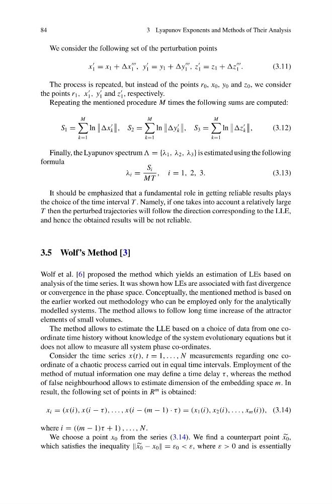
We consider the following set of the perturbation points
x
1 = x 1 + x
1 , y
1 = y 1 + y
1 , z
1 = z 1 + z
1 .
(3.11)
The process is repeated, but instead of the points r 0 , x 0 , y 0 and z 0 , we consider
the points r 1 , x
1 , y
1 and z
1 , respectively.
Repeating the mentioned procedure M times the following sums are computed:
S 1 =
M
k=1
ln
x
k
, S 2 =
M
k=1
ln
y
k
, S 3 =
M
k=1
ln
z
k
,
(3.12)
Finally, the Lyapunov spectrum = {λ 1 , λ 2 , λ 3 } is estimated using the following
formula
λ i =
S i
MT
, i = 1, 2, 3.
(3.13)
It should be emphasized that a fundamental role in getting reliable results plays
the choice of the time interval T . Namely, if one takes into account a relatively large
T then the perturbed trajectories will follow the direction corresponding to the LLE,
and hence the obtained results will be not reliable.
3.5 Wolf’s Method [3]
Wolf et al. [6] proposed the method which yields an estimation of LEs based on
analysis of the time series. It was shown how LEs are associated with fast divergence
or convergence in the phase space. Conceptually, the mentioned method is based on
the earlier worked out methodology who can be employed only for the analytically
modelled systems. The method allows to follow long time increase of the attractor
elements of small volumes.
The method allows to estimate the LLE based on a choice of data from one coordinate time history without knowledge of the system evolutionary equations but it
does not allow to measure all system phase co-ordinates.
Consider the time series x(t), t = 1, . . . , N measurements regarding one coordinate of a chaotic process carried out in equal time intervals. Employment of the
method of mutual information one may define a time delay τ , whereas the method
of false neighbourhood allows to estimate dimension of the embedding space m. In
result, the following set of points in R
m is obtained:
x i = (x(i), x(i − τ ), . . . , x(i − (m − 1) · τ ) = (x 1 (i), x 2 (i), . . . , x m (i)), (3.14)
where i = ((m − 1)τ + 1) , . . . , N .
We choose a point x 0 from the series (3.14). We find a counterpart point
x 0 ,
which satisfies the inequality x 0 − x 0 = ε 0 < ε, where ε > 0 and is essentially
3 Lyapunov Exponents and Methods of Their Analysis
We consider the following set of the perturbation points
x
1 = x 1 + x
1 , y
1 = y 1 + y
1 , z
1 = z 1 + z
1 .
(3.11)
The process is repeated, but instead of the points r 0 , x 0 , y 0 and z 0 , we consider
the points r 1 , x
1 , y
1 and z
1 , respectively.
Repeating the mentioned procedure M times the following sums are computed:
S 1 =
M
k=1
ln
x
k
, S 2 =
M
k=1
ln
y
k
, S 3 =
M
k=1
ln
z
k
,
(3.12)
Finally, the Lyapunov spectrum = {λ 1 , λ 2 , λ 3 } is estimated using the following
formula
λ i =
S i
MT
, i = 1, 2, 3.
(3.13)
It should be emphasized that a fundamental role in getting reliable results plays
the choice of the time interval T . Namely, if one takes into account a relatively large
T then the perturbed trajectories will follow the direction corresponding to the LLE,
and hence the obtained results will be not reliable.
3.5 Wolf’s Method [3]
Wolf et al. [6] proposed the method which yields an estimation of LEs based on
analysis of the time series. It was shown how LEs are associated with fast divergence
or convergence in the phase space. Conceptually, the mentioned method is based on
the earlier worked out methodology who can be employed only for the analytically
modelled systems. The method allows to follow long time increase of the attractor
elements of small volumes.
The method allows to estimate the LLE based on a choice of data from one coordinate time history without knowledge of the system evolutionary equations but it
does not allow to measure all system phase co-ordinates.
Consider the time series x(t), t = 1, . . . , N measurements regarding one coordinate of a chaotic process carried out in equal time intervals. Employment of the
method of mutual information one may define a time delay τ , whereas the method
of false neighbourhood allows to estimate dimension of the embedding space m. In
result, the following set of points in R
m is obtained:
x i = (x(i), x(i − τ ), . . . , x(i − (m − 1) · τ ) = (x 1 (i), x 2 (i), . . . , x m (i)), (3.14)
where i = ((m − 1)τ + 1) , . . . , N .
We choose a point x 0 from the series (3.14). We find a counterpart point
x 0 ,
which satisfies the inequality x 0 − x 0 = ε 0 < ε, where ε > 0 and is essentially