

240
F. de Monte and G. D’Alessandro
4 Estimation Procedure and Optimal Experiment Design
The parameter estimation (PE) technique is based on the minimization of the ordinary
least square (OLS) norm. This leads to the following recursive expression [14]
p
(k+1)
= p
(k)
+ A
(k) X
T(k)
Y − T
(k)
(6a)
where k is the iteration index, p denotes the estimated parameter vector (in the
current case p
T
= [ k C ]), Y is the measured temperature vector, T is the calculated
temperature vector and X is the sensitivity coefficient matrix. Also,
A
(k)
=
X
T(k) X
(k)
−1
(6b)
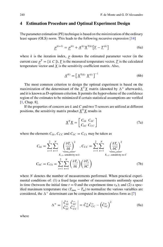
The most common criterion to design the optimal experiment is based on the
maximization of the determinant of the X
T X matrix (denoted by
+ afterwards),
and it is known as D-optimum criterion. It permits the hypervolume of the confidence
region of the estimates to be minimized if certain statistical assumptions are verified
[1, Chap. 8].
If the properties of concern are k and C and two T-sensors are utilized at different
positions, the sensitivity matrix product X
T X results in
X
T X =
C kk C kC
C kC C CC
(7a)
where the elements C kk , C CC and C kC = C Ck may be taken as
C kk =
2
s=1
N
n=1
∂ T s
∂k
2
X s,k , sensitivity to k
, C CC =
2
s=1
N
n=1
∂ T s
∂C
2
X s,C , sensitivity to C
C kC = C Ck =
2
s=1
N
n=1
∂ T s
∂k
∂ T s
∂C
(7b)
where N denotes the number of measurements performed. When practical experimental conditions of: (1) a fixed large number of measurements uniformly spaced
in time (between the initial time t = 0 and the experiment time t N ); and (2) a specified maximum temperature rise (T max − T in ) to normalize the various variables are
considered, the
+ determinant can be computed in dimensionless form as [7]
+
=
˜
C
+
kk
˜
C
+
kC
˜
C
+
kC
˜
C
+
CC
= ˜
C
+
kk
˜
C
+
CC −
˜
C
+
kC
2
(8a)
where
F. de Monte and G. D’Alessandro
4 Estimation Procedure and Optimal Experiment Design
The parameter estimation (PE) technique is based on the minimization of the ordinary
least square (OLS) norm. This leads to the following recursive expression [14]
p
(k+1)
= p
(k)
+ A
(k) X
T(k)
Y − T
(k)
(6a)
where k is the iteration index, p denotes the estimated parameter vector (in the
current case p
T
= [ k C ]), Y is the measured temperature vector, T is the calculated
temperature vector and X is the sensitivity coefficient matrix. Also,
A
(k)
=
X
T(k) X
(k)
−1
(6b)
The most common criterion to design the optimal experiment is based on the
maximization of the determinant of the X
T X matrix (denoted by
+ afterwards),
and it is known as D-optimum criterion. It permits the hypervolume of the confidence
region of the estimates to be minimized if certain statistical assumptions are verified
[1, Chap. 8].
If the properties of concern are k and C and two T-sensors are utilized at different
positions, the sensitivity matrix product X
T X results in
X
T X =
C kk C kC
C kC C CC
(7a)
where the elements C kk , C CC and C kC = C Ck may be taken as
C kk =
2
s=1
N
n=1
∂ T s
∂k
2
X s,k , sensitivity to k
, C CC =
2
s=1
N
n=1
∂ T s
∂C
2
X s,C , sensitivity to C
C kC = C Ck =
2
s=1
N
n=1
∂ T s
∂k
∂ T s
∂C
(7b)
where N denotes the number of measurements performed. When practical experimental conditions of: (1) a fixed large number of measurements uniformly spaced
in time (between the initial time t = 0 and the experiment time t N ); and (2) a specified maximum temperature rise (T max − T in ) to normalize the various variables are
considered, the
+ determinant can be computed in dimensionless form as [7]
+
=
˜
C
+
kk
˜
C
+
kC
˜
C
+
kC
˜
C
+
CC
= ˜
C
+
kk
˜
C
+
CC −
˜
C
+
kC
2
(8a)
where