

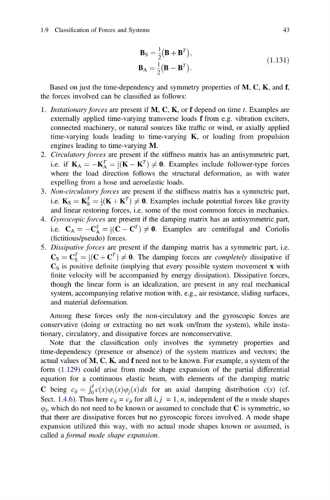
B S ¼
1
2
B þ B
T
À
Á ;
B A ¼
1
2
B À B
T
À
Á :
ð1:131Þ
Based on just the time-dependency and symmetry properties of M, C, K, and f,
the forces involved can be classified as follows:
1. Instationary forces are present if M, C, K, or f depend on time t. Examples are
externally applied time-varying transverse loads f from e.g. vibration exciters,
connected machinery, or natural sources like traffic or wind, or axially applied
time-varying loads leading to time-varying K, or loading from propulsion
engines leading to time-varying M.
2. Circulatory forces are present if the stiffness matrix has an antisymmetric part,
i.e. if K A ¼ ÀK
T
A ¼
1
2 ðK À K
T
Þ 6 ¼ 0: Examples include follower-type forces
where the load direction follows the structural deformation, as with water
expelling from a hose and aeroelastic loads.
3. Non-circulatory forces are present if the stiffness matrix has a symmetric part,
i.e. K S ¼ K
T
S ¼
1
2 ðK þ K
T
Þ 6 ¼ 0: Examples include potential forces like gravity
and linear restoring forces, i.e. some of the most common forces in mechanics.
4. Gyroscopic forces are present if the damping matrix has an antisymmetric part,
i.e. C A ¼ ÀC
T
A ¼
1
2 ðC À C
T
Þ 6 ¼ 0: Examples are centrifugal and Coriolis
(fictitious/pseudo) forces.
5. Dissipative forces are present if the damping matrix has a symmetric part, i.e.
C S ¼ C
T
S ¼
1
2 ðC þ C
T
Þ 6 ¼ 0: The damping forces are completely dissipative if
C S is positive definite (implying that every possible system movement x with
finite velocity will be accompanied by energy dissipation). Dissipative forces,
though the linear form is an idealization, are present in any real mechanical
system, accompanying relative motion with, e.g., air resistance, sliding surfaces,
and material deformation.
Among these forces only the non-circulatory and the gyroscopic forces are
conservative (doing or extracting no net work on/from the system), while instationary, circulatory, and dissipative forces are nonconservative.
Note that the classification only involves the symmetry properties and
time-dependency (presence or absence) of the system matrices and vectors; the
actual values of M, C, K, and f need not to be known. For example, a system of the
form (1.129) could arise from mode shape expansion of the partial differential
equation for a continuous elastic beam, with elements of the damping matric
C being c ij ¼
R l
0 cðxÞu i ðxÞu j ðxÞdx for an axial damping distribution c(x) (cf.
Sect. 1.4.6). Thus here c ij = c ji for all i, j = 1, n, independent of the n mode shapes
u j , which do not need to be known or assumed to conclude that C is symmetric, so
that there are dissipative forces but no gyroscopic forces involved. A mode shape
expansion utilized this way, with no actual mode shapes known or assumed, is
called a formal mode shape expansion.
1.9 Classification of Forces and Systems
43
1
2
B þ B
T
À
Á ;
B A ¼
1
2
B À B
T
À
Á :
ð1:131Þ
Based on just the time-dependency and symmetry properties of M, C, K, and f,
the forces involved can be classified as follows:
1. Instationary forces are present if M, C, K, or f depend on time t. Examples are
externally applied time-varying transverse loads f from e.g. vibration exciters,
connected machinery, or natural sources like traffic or wind, or axially applied
time-varying loads leading to time-varying K, or loading from propulsion
engines leading to time-varying M.
2. Circulatory forces are present if the stiffness matrix has an antisymmetric part,
i.e. if K A ¼ ÀK
T
A ¼
1
2 ðK À K
T
Þ 6 ¼ 0: Examples include follower-type forces
where the load direction follows the structural deformation, as with water
expelling from a hose and aeroelastic loads.
3. Non-circulatory forces are present if the stiffness matrix has a symmetric part,
i.e. K S ¼ K
T
S ¼
1
2 ðK þ K
T
Þ 6 ¼ 0: Examples include potential forces like gravity
and linear restoring forces, i.e. some of the most common forces in mechanics.
4. Gyroscopic forces are present if the damping matrix has an antisymmetric part,
i.e. C A ¼ ÀC
T
A ¼
1
2 ðC À C
T
Þ 6 ¼ 0: Examples are centrifugal and Coriolis
(fictitious/pseudo) forces.
5. Dissipative forces are present if the damping matrix has a symmetric part, i.e.
C S ¼ C
T
S ¼
1
2 ðC þ C
T
Þ 6 ¼ 0: The damping forces are completely dissipative if
C S is positive definite (implying that every possible system movement x with
finite velocity will be accompanied by energy dissipation). Dissipative forces,
though the linear form is an idealization, are present in any real mechanical
system, accompanying relative motion with, e.g., air resistance, sliding surfaces,
and material deformation.
Among these forces only the non-circulatory and the gyroscopic forces are
conservative (doing or extracting no net work on/from the system), while instationary, circulatory, and dissipative forces are nonconservative.
Note that the classification only involves the symmetry properties and
time-dependency (presence or absence) of the system matrices and vectors; the
actual values of M, C, K, and f need not to be known. For example, a system of the
form (1.129) could arise from mode shape expansion of the partial differential
equation for a continuous elastic beam, with elements of the damping matric
C being c ij ¼
R l
0 cðxÞu i ðxÞu j ðxÞdx for an axial damping distribution c(x) (cf.
Sect. 1.4.6). Thus here c ij = c ji for all i, j = 1, n, independent of the n mode shapes
u j , which do not need to be known or assumed to conclude that C is symmetric, so
that there are dissipative forces but no gyroscopic forces involved. A mode shape
expansion utilized this way, with no actual mode shapes known or assumed, is
called a formal mode shape expansion.
1.9 Classification of Forces and Systems
43