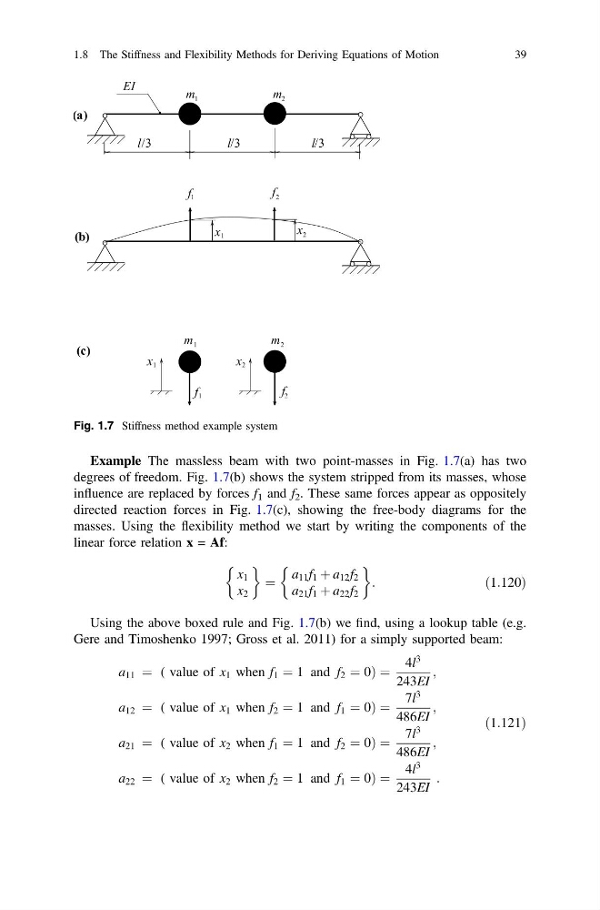
Example The massless beam with two point-masses in Fig. 1.7(a) has two
degrees of freedom. Fig. 1.7(b) shows the system stripped from its masses, whose
influence are replaced by forces f 1 and f 2 . These same forces appear as oppositely
directed reaction forces in Fig. 1.7(c), showing the free-body diagrams for the
masses. Using the flexibility method we start by writing the components of the
linear force relation x = Af:
x 1
x 2
& '
¼
a 11 f 1 þ a 12 f 2
a 21 f 1 þ a 22 f 2
&
'
:
ð1:120Þ
Using the above boxed rule and Fig. 1.7(b) we find, using a lookup table (e.g.
Gere and Timoshenko 1997; Gross et al. 2011) for a simply supported beam:
a 11 ¼ ( value of x 1 when f 1 ¼ 1 and f 2 ¼ 0Þ ¼
4l
3
243EI
;
a 12 ¼ ( value of x 1 when f 2 ¼ 1 and f 1 ¼ 0Þ ¼
7l
3
486EI
;
a 21 ¼ ( value of x 2 when f 1 ¼ 1 and f 2 ¼ 0Þ ¼
7l
3
486EI
;
a 22 ¼ ( value of x 2 when f 2 ¼ 1 and f 1 ¼ 0Þ ¼
4l
3
243EI
:
ð1:121Þ
Fig. 1.7 Stiffness method example system
1.8 The Stiffness and Flexibility Methods for Deriving Equations of Motion
39