

element, such that the magnitude of axial force is partly determined by real-time
measurements of the shaft vibrations. Your task is to analyze possible dynamic
responses of this extended system.
B.1.1 Mathematical Model
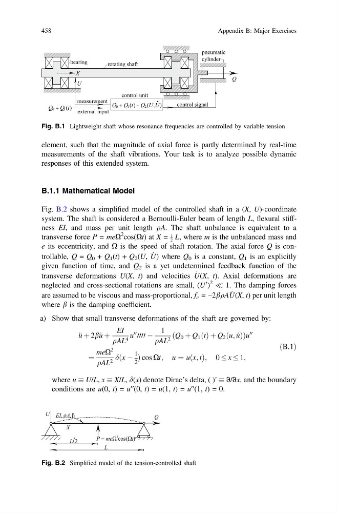
Fig. B.2 shows a simplified model of the controlled shaft in a (X, U)-coordinate
system. The shaft is considered a Bernoulli-Euler beam of length L, flexural stiffness EI, and mass per unit length qA. The shaft unbalance is equivalent to a
transverse force P = meX
2 cos(Xt) at X =
1
2 L, where m is the unbalanced mass and
e its eccentricity, and X is the speed of shaft rotation. The axial force Q is controllable, Q = Q 0 + Q 1 (t) + Q 2 (U, _
U) where Q 0 is a constant, Q 1 is an explicitly
given function of time, and Q 2 is a yet undetermined feedback function of the
transverse deformations U(X, t) and velocities _
U(X, t). Axial deformations are
neglected and cross-sectional rotations are small, (U
0 )
2 ( 1. The damping forces
are assumed to be viscous and mass-proportional, f c = –2bqA _
U(X, t) per unit length
where b is the damping coefficient.
a) Show that small transverse deformations of the shaft are governed by:
€ u þ 2b _
u þ
EI
qAL 4 u
00
0000 À
1
qAL 2 Q 0 þ Q 1 ðtÞ þ Q 2 ðu; _
uÞ
ð
Þ u
00
¼
meX
2
qAL 2 dðx À
1
2
Þ cos Xt; u ¼ uðx; tÞ; 0 x 1;
ðB:1Þ
where u U/L, x X/L, d(x) denote Dirac’s delta, ( )′ ∂/∂x, and the boundary
conditions are u(0, t) = u′′(0, t) = u(1, t) = u′′(1, t) = 0.
Fig. B.1 Lightweight shaft whose resonance frequencies are controlled by variable tension
Fig. B.2 Simplified model of the tension-controlled shaft
458
Appendix B: Major Exercises
measurements of the shaft vibrations. Your task is to analyze possible dynamic
responses of this extended system.
B.1.1 Mathematical Model
Fig. B.2 shows a simplified model of the controlled shaft in a (X, U)-coordinate
system. The shaft is considered a Bernoulli-Euler beam of length L, flexural stiffness EI, and mass per unit length qA. The shaft unbalance is equivalent to a
transverse force P = meX
2 cos(Xt) at X =
1
2 L, where m is the unbalanced mass and
e its eccentricity, and X is the speed of shaft rotation. The axial force Q is controllable, Q = Q 0 + Q 1 (t) + Q 2 (U, _
U) where Q 0 is a constant, Q 1 is an explicitly
given function of time, and Q 2 is a yet undetermined feedback function of the
transverse deformations U(X, t) and velocities _
U(X, t). Axial deformations are
neglected and cross-sectional rotations are small, (U
0 )
2 ( 1. The damping forces
are assumed to be viscous and mass-proportional, f c = –2bqA _
U(X, t) per unit length
where b is the damping coefficient.
a) Show that small transverse deformations of the shaft are governed by:
€ u þ 2b _
u þ
EI
qAL 4 u
00
0000 À
1
qAL 2 Q 0 þ Q 1 ðtÞ þ Q 2 ðu; _
uÞ
ð
Þ u
00
¼
meX
2
qAL 2 dðx À
1
2
Þ cos Xt; u ¼ uðx; tÞ; 0 x 1;
ðB:1Þ
where u U/L, x X/L, d(x) denote Dirac’s delta, ( )′ ∂/∂x, and the boundary
conditions are u(0, t) = u′′(0, t) = u(1, t) = u′′(1, t) = 0.
Fig. B.1 Lightweight shaft whose resonance frequencies are controlled by variable tension
Fig. B.2 Simplified model of the tension-controlled shaft
458
Appendix B: Major Exercises