

A.3. Interfacing with the ODE-Solver
There are many ways to design a user-friendly and flexible interface to the
ODE-solver. It should be easy to adapt to different mathematical models, allow for
easy experimentation with varying system parameters, and aid in verification of
analytical and experimental results.
Commercial simulation software exists that allows the user to define a dynamical
system in a graphical environment, to integrate the equations, and to display features of the result; examples are MATLAB/SIMULINK and SIMULATIONX (formerly
ITI-SIM). However, user-friendliness to general users necessarily implies a lack of
flexibility to satisfy individual needs. Some users find that they will have to code
their own analysis environment, either in high-level general programming languages such as Python, Fortran, C, or C++, and graphical libraries such as OPENGL
– or in dedicated numerically oriented languages such as plane MATLAB and GNU
OCTAVE. In many cases the latter will provide an efficient and satisfactory compromise between the conflicting requirements of short program development time
and ease of use on the one side, and flexibility and high-speed computing on the
other.
If you consider programming your own simulation software, a starting point
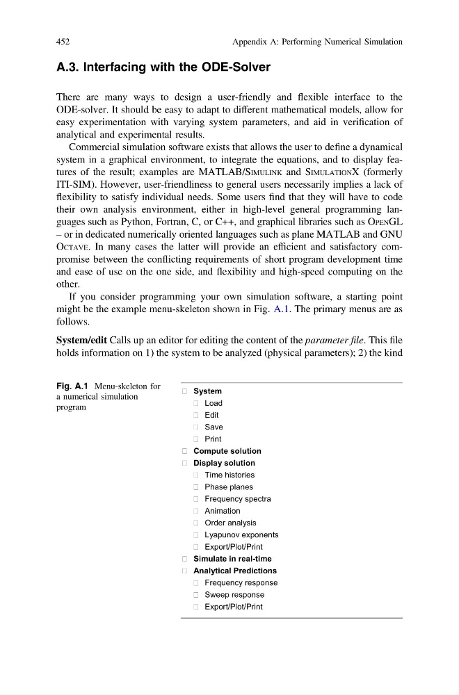
might be the example menu-skeleton shown in Fig. A.1. The primary menus are as
follows.
System/edit Calls up an editor for editing the content of the parameter file. This file
holds information on 1) the system to be analyzed (physical parameters); 2) the kind
System
Load
Edit
Save
Print
Compute solution
Display solution
Time histories
Phase planes
Frequency spectra
Animation
Order analysis
Lyapunov exponents
Export/Plot/Print
Simulate in real-time
Analytical Predictions
Frequency response
Sweep response
Export/Plot/Print
Fig. A.1 Menu-skeleton for
a numerical simulation
program
452
Appendix A: Performing Numerical Simulation
There are many ways to design a user-friendly and flexible interface to the
ODE-solver. It should be easy to adapt to different mathematical models, allow for
easy experimentation with varying system parameters, and aid in verification of
analytical and experimental results.
Commercial simulation software exists that allows the user to define a dynamical
system in a graphical environment, to integrate the equations, and to display features of the result; examples are MATLAB/SIMULINK and SIMULATIONX (formerly
ITI-SIM). However, user-friendliness to general users necessarily implies a lack of
flexibility to satisfy individual needs. Some users find that they will have to code
their own analysis environment, either in high-level general programming languages such as Python, Fortran, C, or C++, and graphical libraries such as OPENGL
– or in dedicated numerically oriented languages such as plane MATLAB and GNU
OCTAVE. In many cases the latter will provide an efficient and satisfactory compromise between the conflicting requirements of short program development time
and ease of use on the one side, and flexibility and high-speed computing on the
other.
If you consider programming your own simulation software, a starting point
might be the example menu-skeleton shown in Fig. A.1. The primary menus are as
follows.
System/edit Calls up an editor for editing the content of the parameter file. This file
holds information on 1) the system to be analyzed (physical parameters); 2) the kind
System
Load
Edit
Save
Compute solution
Display solution
Time histories
Phase planes
Frequency spectra
Animation
Order analysis
Lyapunov exponents
Export/Plot/Print
Simulate in real-time
Analytical Predictions
Frequency response
Sweep response
Export/Plot/Print
Fig. A.1 Menu-skeleton for
a numerical simulation
program
452
Appendix A: Performing Numerical Simulation