

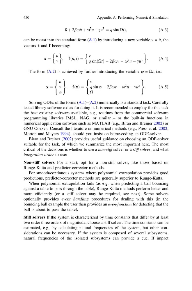
€ u þ 2bx _
u þ x
2 u þ cu
3
¼ q sinðXtÞ;
ðA:3Þ
can be recast into the standard form (A.1) by introducing a new variable v = _
u, the
vectors ~ x and ~ f becoming:
~ x ¼
u
v
& '
; ~ fðx; tÞ ¼
v
q sinðXtÞ À 2bxv À x
2 u À cu
3
&
'
:
ðA:4Þ
The form (A.2) is achieved by further introducing the variable u = Xt, i.e.:
x ¼
u
v
u
8
<
:
9
=
;
; fðxÞ ¼
v
q sin u À 2bxv À x
2 u À cu
3
X
8
<
:
9
=
;
:
ðA:5Þ
Solving ODEs of the forms (A.1)–(A.2) numerically is a standard task. Carefully
tested library software exists for doing it. It is recommended to employ for this task
the best existing software available, e.g., routines from the commercial software
programming libraries IMSL, NAG, or similar – or the built-in functions in
numerical application software such as MATLAB (e.g., Biran and Breiner 2002) or
GNU OCTAVE. Consult the literature on numerical methods (e.g., Press et al. 2002;
Morton and Mayers 1994), should you insist on home-coding an ODE-solver.
Biran and Breiner (2002) provides useful guidance on choosing an ODE-solver
suitable for the task, of which we summarize the most important here. The most
critical of the decisions is whether to use a non-stiff solver or a stiff solver, and what
integration order to use:
Non-stiff solvers For a start, opt for a non-stiff solver, like those based on
Runge-Kutta and predictor-corrector methods.
For smooth/continuous systems where polynomial extrapolation provides good
predictions, predictor-corrector methods are generally superior to Runge-Kutta.
When polynomial extrapolation fails (as e.g. when predicting a ball bouncing
against a table to pass through the table), Runge-Kutta methods perform better and
more efficiently (or a stiff solver may be required, see next). Some solvers
optionally provides event handling procedures for dealing with this (in the
bouncing ball example the user then provides an even-function for detecting that the
ball is about to pass the table).
Stiff solvers If the system is characterized by time constants that differ by at least
two order three orders of magnitude, choose a stiff solver. The time constants can be
estimated, e.g., by calculating natural frequencies of the system, but other considerations can be necessary. If the system is composed of several subsystems,
natural frequencies of the isolated subsystems can provide a cue. If impact
450
Appendix A: Performing Numerical Simulation
u þ x
2 u þ cu
3
¼ q sinðXtÞ;
ðA:3Þ
can be recast into the standard form (A.1) by introducing a new variable v = _
u, the
vectors ~ x and ~ f becoming:
~ x ¼
u
v
& '
; ~ fðx; tÞ ¼
v
q sinðXtÞ À 2bxv À x
2 u À cu
3
&
'
:
ðA:4Þ
The form (A.2) is achieved by further introducing the variable u = Xt, i.e.:
x ¼
u
v
u
8
<
:
9
=
;
; fðxÞ ¼
v
q sin u À 2bxv À x
2 u À cu
3
X
8
<
:
9
=
;
:
ðA:5Þ
Solving ODEs of the forms (A.1)–(A.2) numerically is a standard task. Carefully
tested library software exists for doing it. It is recommended to employ for this task
the best existing software available, e.g., routines from the commercial software
programming libraries IMSL, NAG, or similar – or the built-in functions in
numerical application software such as MATLAB (e.g., Biran and Breiner 2002) or
GNU OCTAVE. Consult the literature on numerical methods (e.g., Press et al. 2002;
Morton and Mayers 1994), should you insist on home-coding an ODE-solver.
Biran and Breiner (2002) provides useful guidance on choosing an ODE-solver
suitable for the task, of which we summarize the most important here. The most
critical of the decisions is whether to use a non-stiff solver or a stiff solver, and what
integration order to use:
Non-stiff solvers For a start, opt for a non-stiff solver, like those based on
Runge-Kutta and predictor-corrector methods.
For smooth/continuous systems where polynomial extrapolation provides good
predictions, predictor-corrector methods are generally superior to Runge-Kutta.
When polynomial extrapolation fails (as e.g. when predicting a ball bouncing
against a table to pass through the table), Runge-Kutta methods perform better and
more efficiently (or a stiff solver may be required, see next). Some solvers
optionally provides event handling procedures for dealing with this (in the
bouncing ball example the user then provides an even-function for detecting that the
ball is about to pass the table).
Stiff solvers If the system is characterized by time constants that differ by at least
two order three orders of magnitude, choose a stiff solver. The time constants can be
estimated, e.g., by calculating natural frequencies of the system, but other considerations can be necessary. If the system is composed of several subsystems,
natural frequencies of the isolated subsystems can provide a cue. If impact
450
Appendix A: Performing Numerical Simulation