

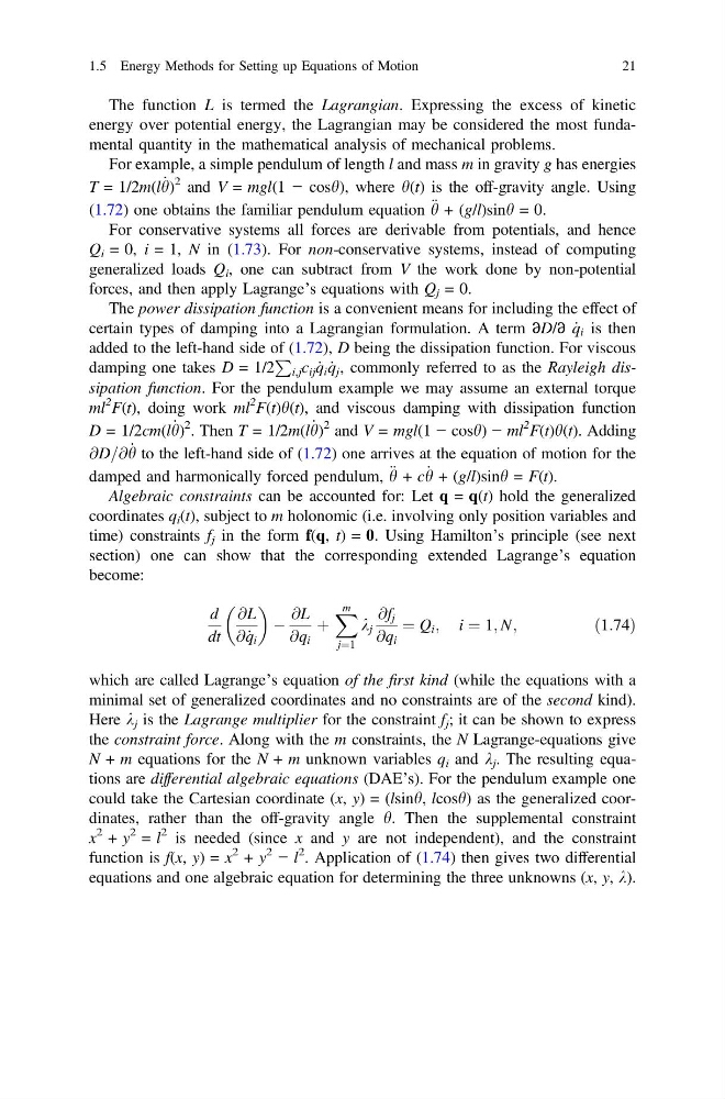
The function L is termed the Lagrangian. Expressing the excess of kinetic
energy over potential energy, the Lagrangian may be considered the most fundamental quantity in the mathematical analysis of mechanical problems.
For example, a simple pendulum of length l and mass m in gravity g has energies
T = 1/2m(l _
h)
2 and V = mgl(1 − cosh), where h(t) is the off-gravity angle. Using
(1.72) one obtains the familiar pendulum equation € h + (g/l)sinh = 0.
For conservative systems all forces are derivable from potentials, and hence
Q i = 0, i = 1, N in (1.73). For non-conservative systems, instead of computing
generalized loads Q i , one can subtract from V the work done by non-potential
forces, and then apply Lagrange’s equations with Q j = 0.
The power dissipation function is a convenient means for including the effect of
certain types of damping into a Lagrangian formulation. A term ∂D/∂ _
q i is then
added to the left-hand side of (1.72), D being the dissipation function. For viscous
damping one takes D = 1/2
P
i,j c ij _
q i _
q j , commonly referred to as the Rayleigh dissipation function. For the pendulum example we may assume an external torque
ml
2 F(t), doing work ml
2 F(t)h(t), and viscous damping with dissipation function
D = 1/2cm(l _
h)
2 . Then T = 1/2m(l _
h)
2 and V = mgl(1 − cosh) − ml
2 F(t)h(t). Adding
@D=@ _
h to the left-hand side of (1.72) one arrives at the equation of motion for the
damped and harmonically forced pendulum, € h + c _
h + (g/l)sinh = F(t).
Algebraic constraints can be accounted for: Let q = q(t) hold the generalized
coordinates q i (t), subject to m holonomic (i.e. involving only position variables and
time) constraints f j in the form f(q, t) = 0. Using Hamilton’s principle (see next
section) one can show that the corresponding extended Lagrange’s equation
become:
d
dt
@L
@ _
q i
À
@L
@q i
þ
X m
j¼1
k j
@f j
@q i
¼ Q i ; i ¼ 1; N;
ð1:74Þ
which are called Lagrange’s equation of the first kind (while the equations with a
minimal set of generalized coordinates and no constraints are of the second kind).
Here k j is the Lagrange multiplier for the constraint f j ; it can be shown to express
the constraint force. Along with the m constraints, the N Lagrange-equations give
N + m equations for the N + m unknown variables q i and k j . The resulting equations are differential algebraic equations (DAE’s). For the pendulum example one
could take the Cartesian coordinate (x, y) = (lsinh, lcosh) as the generalized coordinates, rather than the off-gravity angle h. Then the supplemental constraint
x
2 + y
2 = l
2 is needed (since x and y are not independent), and the constraint
function is f(x, y) = x
2 + y
2
− l
2 . Application of (1.74) then gives two differential
equations and one algebraic equation for determining the three unknowns (x, y, k).
1.5 Energy Methods for Setting up Equations of Motion
21
energy over potential energy, the Lagrangian may be considered the most fundamental quantity in the mathematical analysis of mechanical problems.
For example, a simple pendulum of length l and mass m in gravity g has energies
T = 1/2m(l _
h)
2 and V = mgl(1 − cosh), where h(t) is the off-gravity angle. Using
(1.72) one obtains the familiar pendulum equation € h + (g/l)sinh = 0.
For conservative systems all forces are derivable from potentials, and hence
Q i = 0, i = 1, N in (1.73). For non-conservative systems, instead of computing
generalized loads Q i , one can subtract from V the work done by non-potential
forces, and then apply Lagrange’s equations with Q j = 0.
The power dissipation function is a convenient means for including the effect of
certain types of damping into a Lagrangian formulation. A term ∂D/∂ _
q i is then
added to the left-hand side of (1.72), D being the dissipation function. For viscous
damping one takes D = 1/2
P
i,j c ij _
q i _
q j , commonly referred to as the Rayleigh dissipation function. For the pendulum example we may assume an external torque
ml
2 F(t), doing work ml
2 F(t)h(t), and viscous damping with dissipation function
D = 1/2cm(l _
h)
2 . Then T = 1/2m(l _
h)
2 and V = mgl(1 − cosh) − ml
2 F(t)h(t). Adding
@D=@ _
h to the left-hand side of (1.72) one arrives at the equation of motion for the
damped and harmonically forced pendulum, € h + c _
h + (g/l)sinh = F(t).
Algebraic constraints can be accounted for: Let q = q(t) hold the generalized
coordinates q i (t), subject to m holonomic (i.e. involving only position variables and
time) constraints f j in the form f(q, t) = 0. Using Hamilton’s principle (see next
section) one can show that the corresponding extended Lagrange’s equation
become:
d
dt
@L
@ _
q i
À
@L
@q i
þ
X m
j¼1
k j
@f j
@q i
¼ Q i ; i ¼ 1; N;
ð1:74Þ
which are called Lagrange’s equation of the first kind (while the equations with a
minimal set of generalized coordinates and no constraints are of the second kind).
Here k j is the Lagrange multiplier for the constraint f j ; it can be shown to express
the constraint force. Along with the m constraints, the N Lagrange-equations give
N + m equations for the N + m unknown variables q i and k j . The resulting equations are differential algebraic equations (DAE’s). For the pendulum example one
could take the Cartesian coordinate (x, y) = (lsinh, lcosh) as the generalized coordinates, rather than the off-gravity angle h. Then the supplemental constraint
x
2 + y
2 = l
2 is needed (since x and y are not independent), and the constraint
function is f(x, y) = x
2 + y
2
− l
2 . Application of (1.74) then gives two differential
equations and one algebraic equation for determining the three unknowns (x, y, k).
1.5 Energy Methods for Setting up Equations of Motion
21