

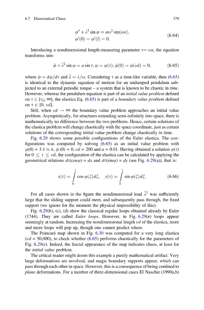
u
00
þ k
2 sin u ¼ ax
2 sinðxsÞ;
u
0
ð0Þ ¼ u
0
ðlÞ ¼ 0:
ð6:64Þ
Introducing a nondimensional length-measuring parameter s¼ xs, the equation
transforms into
€
u þ ~ k
2 sin u ¼ a sin s; u ¼ uðsÞ; _
uð0Þ ¼ _
uðxlÞ ¼ 0;
ð6:65Þ
where _
u ¼ du=ds and ^ k ¼ k=x. Considering s as a time-like variable, then (6.65)
is identical to the dynamic equation of motion for an undamped pendulum subjected to an external periodic torque – a system that is known to be chaotic in time.
However, whereas the pendulum equation is part of an initial value problem defined
on s 2 [s 0 ; ∞[, the elastica Eq. (6.65) is part of a boundary value problem defined
on s 2 [0; xl].
Still, when xl ! ∞ the boundary value problem approaches an initial value
problem. Asymptotically, for structures extending semi-infinitely into space, there is
mathematically no difference between the two problems. Hence, certain solutions of
the elastica problem will change chaotically with the space coordinate, just as certain
solutions of the corresponding initial value problem change chaotically in time.
Fig. 6.29 shows some possible configurations of the Euler elastica. The configurations was computed by solving (6.65) as an initial value problem with
u(0) = 3.1 % p, _
u (0) = 0, xl = 200 and a = 0.01. Having obtained a solution u(s)
for 0
s
xl, the configuration of the elastica can be calculated by applying the
geometrical relations ds(cosu) = dx and ds(sinu) = dy (see Fig. 6.29(a)), that is:
xðsÞ ¼
Z s
0
cos uðnÞdn; yðsÞ ¼
Z s
0
sin uðnÞdn:
ð6:66Þ
For all cases shown in the figure the nondimensional load ~ k
2 was sufficiently
large that the sliding support could meet, and subsequently pass through, the fixed
support (we ignore for the moment the physical impossibility of this).
Fig. 6.29(b), (c), (d) show the classical regular loops obtained already by Euler
(1744). They are called Euler loops. However, in Fig. 6.29(e) loops appear
seemingly at random. Increasing the nondimensional length xl of the elastica, more
and more loops will pop up, though one cannot predict where.
The Poincaré map shown in Fig. 6.30 was computed for a very long elastica
(xl = 50,000), to check whether (6.65) performs chaotically for the parameters of
Fig. 6.29(e). Indeed, the fractal appearance of the map indicates chaos, at least for
the initial value problem.
The critical reader might doom this example a purely mathematical artifact. Very
large deformations are involved, and magic boundary supports appear, which can
pass through each other in space. However, this is a consequence of being confined to
plane deformations. For a number of three-dimensional cases El Naschie (1990a,b)
6.7 Elastostatical Chaos
379
00
þ k
2 sin u ¼ ax
2 sinðxsÞ;
u
0
ð0Þ ¼ u
0
ðlÞ ¼ 0:
ð6:64Þ
Introducing a nondimensional length-measuring parameter s¼ xs, the equation
transforms into
€
u þ ~ k
2 sin u ¼ a sin s; u ¼ uðsÞ; _
uð0Þ ¼ _
uðxlÞ ¼ 0;
ð6:65Þ
where _
u ¼ du=ds and ^ k ¼ k=x. Considering s as a time-like variable, then (6.65)
is identical to the dynamic equation of motion for an undamped pendulum subjected to an external periodic torque – a system that is known to be chaotic in time.
However, whereas the pendulum equation is part of an initial value problem defined
on s 2 [s 0 ; ∞[, the elastica Eq. (6.65) is part of a boundary value problem defined
on s 2 [0; xl].
Still, when xl ! ∞ the boundary value problem approaches an initial value
problem. Asymptotically, for structures extending semi-infinitely into space, there is
mathematically no difference between the two problems. Hence, certain solutions of
the elastica problem will change chaotically with the space coordinate, just as certain
solutions of the corresponding initial value problem change chaotically in time.
Fig. 6.29 shows some possible configurations of the Euler elastica. The configurations was computed by solving (6.65) as an initial value problem with
u(0) = 3.1 % p, _
u (0) = 0, xl = 200 and a = 0.01. Having obtained a solution u(s)
for 0
s
xl, the configuration of the elastica can be calculated by applying the
geometrical relations ds(cosu) = dx and ds(sinu) = dy (see Fig. 6.29(a)), that is:
xðsÞ ¼
Z s
0
cos uðnÞdn; yðsÞ ¼
Z s
0
sin uðnÞdn:
ð6:66Þ
For all cases shown in the figure the nondimensional load ~ k
2 was sufficiently
large that the sliding support could meet, and subsequently pass through, the fixed
support (we ignore for the moment the physical impossibility of this).
Fig. 6.29(b), (c), (d) show the classical regular loops obtained already by Euler
(1744). They are called Euler loops. However, in Fig. 6.29(e) loops appear
seemingly at random. Increasing the nondimensional length xl of the elastica, more
and more loops will pop up, though one cannot predict where.
The Poincaré map shown in Fig. 6.30 was computed for a very long elastica
(xl = 50,000), to check whether (6.65) performs chaotically for the parameters of
Fig. 6.29(e). Indeed, the fractal appearance of the map indicates chaos, at least for
the initial value problem.
The critical reader might doom this example a purely mathematical artifact. Very
large deformations are involved, and magic boundary supports appear, which can
pass through each other in space. However, this is a consequence of being confined to
plane deformations. For a number of three-dimensional cases El Naschie (1990a,b)
6.7 Elastostatical Chaos
379