

€ u þ b _
u þ
1
c 1
u ¼
1
c 2
q cosðXtÞ þ
0
c 3
D
c 4
;
ð6:55Þ
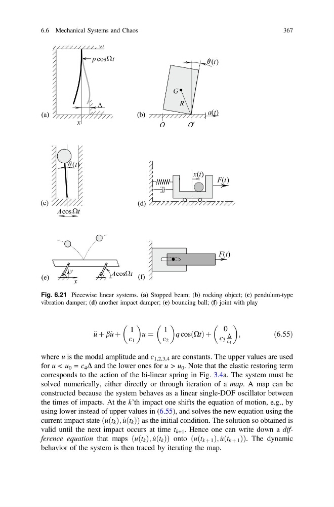
where u is the modal amplitude and c 1,2,3,4 are constants. The upper values are used
for u < u 0 = c 4 D and the lower ones for u > u 0 . Note that the elastic restoring term
corresponds to the action of the bi-linear spring in Fig. 3.4a. The system must be
solved numerically, either directly or through iteration of a map. A map can be
constructed because the system behaves as a linear single-DOF oscillator between
the times of impacts. At the k’th impact one shifts the equation of motion, e.g., by
using lower instead of upper values in (6.55), and solves the new equation using the
current impact state ðuðt k Þ; _
uðt k ÞÞ as the initial condition. The solution so obtained is
valid until the next impact occurs at time t k+1 . Hence one can write down a difference equation that maps ðuðt k Þ; _
uðt k ÞÞ onto ðuðt k þ 1 Þ; _
uðt k þ 1 ÞÞ. The dynamic
behavior of the system is then traced by iterating the map.
Fig. 6.21 Piecewise linear systems. (a) Stopped beam; (b) rocking object; (c) pendulum-type
vibration damper; (d) another impact damper; (e) bouncing ball; (f) joint with play
6.6 Mechanical Systems and Chaos
367
u þ
1
c 1
u ¼
1
c 2
q cosðXtÞ þ
0
c 3
D
c 4
;
ð6:55Þ
where u is the modal amplitude and c 1,2,3,4 are constants. The upper values are used
for u < u 0 = c 4 D and the lower ones for u > u 0 . Note that the elastic restoring term
corresponds to the action of the bi-linear spring in Fig. 3.4a. The system must be
solved numerically, either directly or through iteration of a map. A map can be
constructed because the system behaves as a linear single-DOF oscillator between
the times of impacts. At the k’th impact one shifts the equation of motion, e.g., by
using lower instead of upper values in (6.55), and solves the new equation using the
current impact state ðuðt k Þ; _
uðt k ÞÞ as the initial condition. The solution so obtained is
valid until the next impact occurs at time t k+1 . Hence one can write down a difference equation that maps ðuðt k Þ; _
uðt k ÞÞ onto ðuðt k þ 1 Þ; _
uðt k þ 1 ÞÞ. The dynamic
behavior of the system is then traced by iterating the map.
Fig. 6.21 Piecewise linear systems. (a) Stopped beam; (b) rocking object; (c) pendulum-type
vibration damper; (d) another impact damper; (e) bouncing ball; (f) joint with play
6.6 Mechanical Systems and Chaos
367