

where V max and T max are, respectively, the maximum potential and kinetic energy
associated with an oscillating field ~ u(x)(sinxt), and ~
x 1 is the Rayleigh quotient
estimate of x 1 . The function ~ u(x) is arbitrary, except that it must be C
2m (2m is the
order of the differential equation), and satisfy the essential boundary conditions
(those having derivatives of order 0, 1, …, m − 1). We shall return to Rayleigh’s
quotient in Chap. 2, defining it there in terms of differential operators.
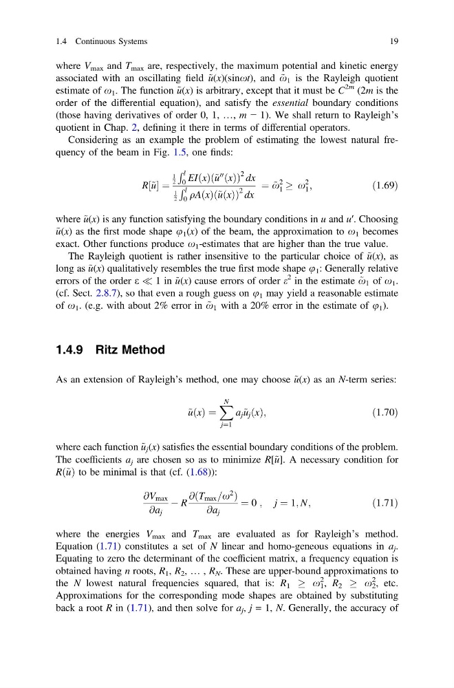
Considering as an example the problem of estimating the lowest natural frequency of the beam in Fig. 1.5, one finds:
R½~ u ¼
1
2
R l
0 EIðxÞ ~ u
00
ðxÞ
ð
Þ
2 dx
1
2
R l
0 qAðxÞ ~ uðxÞ
ð
Þ
2 dx
¼ ~
x
2
1 ! x
2
1 ;
ð1:69Þ
where ~ u(x) is any function satisfying the boundary conditions in u and u′. Choosing
~ u(x) as the first mode shape u 1 (x) of the beam, the approximation to x 1 becomes
exact. Other functions produce x 1 -estimates that are higher than the true value.
The Rayleigh quotient is rather insensitive to the particular choice of ~ u(x), as
long as ~ u(x) qualitatively resembles the true first mode shape u 1 : Generally relative
errors of the order e ( 1 in ~ u(x) cause errors of order e
2 in the estimate ~
x 1 of x 1 .
(cf. Sect. 2.8.7), so that even a rough guess on u 1 may yield a reasonable estimate
of x 1 . (e.g. with about 2% error in ~
x 1 with a 20% error in the estimate of u 1 ).
1.4.9 Ritz Method
As an extension of Rayleigh’s method, one may choose ~ u(x) as an N-term series:
~ uðxÞ ¼
X N
j¼1
a j ~ u j ðxÞ;
ð1:70Þ
where each function ~ u j (x) satisfies the essential boundary conditions of the problem.
The coefficients a j are chosen so as to minimize R[~ u]. A necessary condition for
Rð~ uÞ to be minimal is that (cf. (1.68)):
@V max
@a j
À R
@ T max =x
2
ð
Þ
@a j
¼ 0 ; j ¼ 1; N;
ð1:71Þ
where the energies V max and T max are evaluated as for Rayleigh’s method.
Equation (1.71) constitutes a set of N linear and homo-geneous equations in a j .
Equating to zero the determinant of the coefficient matrix, a frequency equation is
obtained having n roots, R 1 , R 2 , … , R N . These are upper-bound approximations to
the N lowest natural frequencies squared, that is: R 1 ! x 1
2 , R 2 ! x 2
2 , etc.
Approximations for the corresponding mode shapes are obtained by substituting
back a root R in (1.71), and then solve for a j , j = 1, N. Generally, the accuracy of
1.4 Continuous Systems
19
associated with an oscillating field ~ u(x)(sinxt), and ~
x 1 is the Rayleigh quotient
estimate of x 1 . The function ~ u(x) is arbitrary, except that it must be C
2m (2m is the
order of the differential equation), and satisfy the essential boundary conditions
(those having derivatives of order 0, 1, …, m − 1). We shall return to Rayleigh’s
quotient in Chap. 2, defining it there in terms of differential operators.
Considering as an example the problem of estimating the lowest natural frequency of the beam in Fig. 1.5, one finds:
R½~ u ¼
1
2
R l
0 EIðxÞ ~ u
00
ðxÞ
ð
Þ
2 dx
1
2
R l
0 qAðxÞ ~ uðxÞ
ð
Þ
2 dx
¼ ~
x
2
1 ! x
2
1 ;
ð1:69Þ
where ~ u(x) is any function satisfying the boundary conditions in u and u′. Choosing
~ u(x) as the first mode shape u 1 (x) of the beam, the approximation to x 1 becomes
exact. Other functions produce x 1 -estimates that are higher than the true value.
The Rayleigh quotient is rather insensitive to the particular choice of ~ u(x), as
long as ~ u(x) qualitatively resembles the true first mode shape u 1 : Generally relative
errors of the order e ( 1 in ~ u(x) cause errors of order e
2 in the estimate ~
x 1 of x 1 .
(cf. Sect. 2.8.7), so that even a rough guess on u 1 may yield a reasonable estimate
of x 1 . (e.g. with about 2% error in ~
x 1 with a 20% error in the estimate of u 1 ).
1.4.9 Ritz Method
As an extension of Rayleigh’s method, one may choose ~ u(x) as an N-term series:
~ uðxÞ ¼
X N
j¼1
a j ~ u j ðxÞ;
ð1:70Þ
where each function ~ u j (x) satisfies the essential boundary conditions of the problem.
The coefficients a j are chosen so as to minimize R[~ u]. A necessary condition for
Rð~ uÞ to be minimal is that (cf. (1.68)):
@V max
@a j
À R
@ T max =x
2
ð
Þ
@a j
¼ 0 ; j ¼ 1; N;
ð1:71Þ
where the energies V max and T max are evaluated as for Rayleigh’s method.
Equation (1.71) constitutes a set of N linear and homo-geneous equations in a j .
Equating to zero the determinant of the coefficient matrix, a frequency equation is
obtained having n roots, R 1 , R 2 , … , R N . These are upper-bound approximations to
the N lowest natural frequencies squared, that is: R 1 ! x 1
2 , R 2 ! x 2
2 , etc.
Approximations for the corresponding mode shapes are obtained by substituting
back a root R in (1.71), and then solve for a j , j = 1, N. Generally, the accuracy of
1.4 Continuous Systems
19