

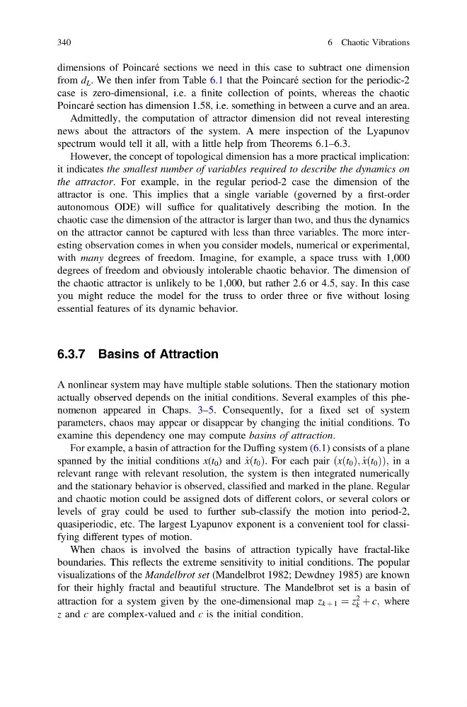
dimensions of Poincaré sections we need in this case to subtract one dimension
from d L . We then infer from Table 6.1 that the Poincaré section for the periodic-2
case is zero-dimensional, i.e. a finite collection of points, whereas the chaotic
Poincaré section has dimension 1.58, i.e. something in between a curve and an area.
Admittedly, the computation of attractor dimension did not reveal interesting
news about the attractors of the system. A mere inspection of the Lyapunov
spectrum would tell it all, with a little help from Theorems 6.1–6.3.
However, the concept of topological dimension has a more practical implication:
it indicates the smallest number of variables required to describe the dynamics on
the attractor. For example, in the regular period-2 case the dimension of the
attractor is one. This implies that a single variable (governed by a first-order
autonomous ODE) will suffice for qualitatively describing the motion. In the
chaotic case the dimension of the attractor is larger than two, and thus the dynamics
on the attractor cannot be captured with less than three variables. The more interesting observation comes in when you consider models, numerical or experimental,
with many degrees of freedom. Imagine, for example, a space truss with 1,000
degrees of freedom and obviously intolerable chaotic behavior. The dimension of
the chaotic attractor is unlikely to be 1,000, but rather 2.6 or 4.5, say. In this case
you might reduce the model for the truss to order three or five without losing
essential features of its dynamic behavior.
6.3.7 Basins of Attraction
A nonlinear system may have multiple stable solutions. Then the stationary motion
actually observed depends on the initial conditions. Several examples of this phenomenon appeared in Chaps. 3–5. Consequently, for a fixed set of system
parameters, chaos may appear or disappear by changing the initial conditions. To
examine this dependency one may compute basins of attraction.
For example, a basin of attraction for the Duffing system (6.1) consists of a plane
spanned by the initial conditions x(t 0 ) and _
xðt 0 Þ. For each pair ðxðt 0 Þ; _
xðt 0 ÞÞ; in a
relevant range with relevant resolution, the system is then integrated numerically
and the stationary behavior is observed, classified and marked in the plane. Regular
and chaotic motion could be assigned dots of different colors, or several colors or
levels of gray could be used to further sub-classify the motion into period-2,
quasiperiodic, etc. The largest Lyapunov exponent is a convenient tool for classifying different types of motion.
When chaos is involved the basins of attraction typically have fractal-like
boundaries. This reflects the extreme sensitivity to initial conditions. The popular
visualizations of the Mandelbrot set (Mandelbrot 1982; Dewdney 1985) are known
for their highly fractal and beautiful structure. The Mandelbrot set is a basin of
attraction for a system given by the one-dimensional map z k þ 1 ¼ z
2
k þ c; where
z and c are complex-valued and c is the initial condition.
340
6 Chaotic Vibrations
from d L . We then infer from Table 6.1 that the Poincaré section for the periodic-2
case is zero-dimensional, i.e. a finite collection of points, whereas the chaotic
Poincaré section has dimension 1.58, i.e. something in between a curve and an area.
Admittedly, the computation of attractor dimension did not reveal interesting
news about the attractors of the system. A mere inspection of the Lyapunov
spectrum would tell it all, with a little help from Theorems 6.1–6.3.
However, the concept of topological dimension has a more practical implication:
it indicates the smallest number of variables required to describe the dynamics on
the attractor. For example, in the regular period-2 case the dimension of the
attractor is one. This implies that a single variable (governed by a first-order
autonomous ODE) will suffice for qualitatively describing the motion. In the
chaotic case the dimension of the attractor is larger than two, and thus the dynamics
on the attractor cannot be captured with less than three variables. The more interesting observation comes in when you consider models, numerical or experimental,
with many degrees of freedom. Imagine, for example, a space truss with 1,000
degrees of freedom and obviously intolerable chaotic behavior. The dimension of
the chaotic attractor is unlikely to be 1,000, but rather 2.6 or 4.5, say. In this case
you might reduce the model for the truss to order three or five without losing
essential features of its dynamic behavior.
6.3.7 Basins of Attraction
A nonlinear system may have multiple stable solutions. Then the stationary motion
actually observed depends on the initial conditions. Several examples of this phenomenon appeared in Chaps. 3–5. Consequently, for a fixed set of system
parameters, chaos may appear or disappear by changing the initial conditions. To
examine this dependency one may compute basins of attraction.
For example, a basin of attraction for the Duffing system (6.1) consists of a plane
spanned by the initial conditions x(t 0 ) and _
xðt 0 Þ. For each pair ðxðt 0 Þ; _
xðt 0 ÞÞ; in a
relevant range with relevant resolution, the system is then integrated numerically
and the stationary behavior is observed, classified and marked in the plane. Regular
and chaotic motion could be assigned dots of different colors, or several colors or
levels of gray could be used to further sub-classify the motion into period-2,
quasiperiodic, etc. The largest Lyapunov exponent is a convenient tool for classifying different types of motion.
When chaos is involved the basins of attraction typically have fractal-like
boundaries. This reflects the extreme sensitivity to initial conditions. The popular
visualizations of the Mandelbrot set (Mandelbrot 1982; Dewdney 1985) are known
for their highly fractal and beautiful structure. The Mandelbrot set is a basin of
attraction for a system given by the one-dimensional map z k þ 1 ¼ z
2
k þ c; where
z and c are complex-valued and c is the initial condition.
340
6 Chaotic Vibrations