

Lyapunov exponents quantify the average rate at which information degrades.
Defined in terms of the base-2 logarithm, cf. (6.4), Lyapunov exponents are measured in bit/second.
Reconsidering the chaotic Duffing equation, we obtained at the end of
Sect. 6.3.4 an estimate of the largest Lyapunov exponent, ^ k 1 % 0:19. Hence, with
initial conditions specified to within an accuracy of one part per million (20 bits), all
bits of information will be lost after (20 bits)/(0.19 bits/second) % 105 s, corresponding to approximately 20 periods of the driving force when X = 1.2. Beyond
this time – the horizon of predictability – nothing will be known about the state of
the system, except than it would be somewhere on the chaotic attractor.
Generally, if the numerical or experimental accuracy is of the order 10
−m , then
the time horizon for reasonable predictions is of the order
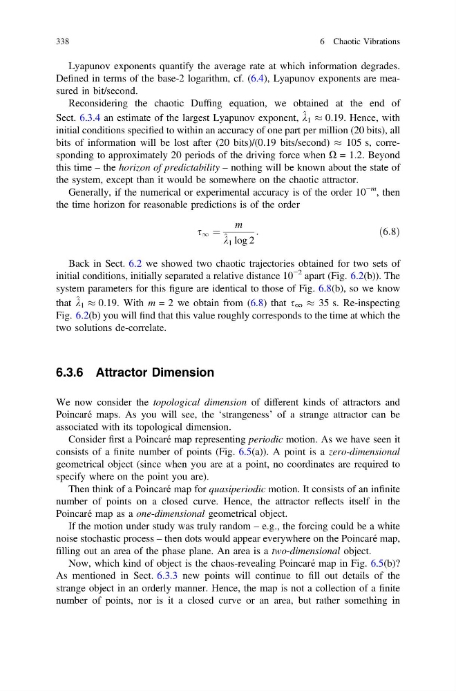
s 1 ¼
m
^ k 1 log 2
:
ð6:8Þ
Back in Sect. 6.2 we showed two chaotic trajectories obtained for two sets of
initial conditions, initially separated a relative distance 10
−2 apart (Fig. 6.2(b)). The
system parameters for this figure are identical to those of Fig. 6.8(b), so we know
that ^ k 1 % 0:19. With m = 2 we obtain from (6.8) that s ∞ % 35 s. Re-inspecting
Fig. 6.2(b) you will find that this value roughly corresponds to the time at which the
two solutions de-correlate.
6.3.6 Attractor Dimension
We now consider the topological dimension of different kinds of attractors and
Poincaré maps. As you will see, the ‘strangeness’ of a strange attractor can be
associated with its topological dimension.
Consider first a Poincaré map representing periodic motion. As we have seen it
consists of a finite number of points (Fig. 6.5(a)). A point is a zero-dimensional
geometrical object (since when you are at a point, no coordinates are required to
specify where on the point you are).
Then think of a Poincaré map for quasiperiodic motion. It consists of an infinite
number of points on a closed curve. Hence, the attractor reflects itself in the
Poincaré map as a one-dimensional geometrical object.
If the motion under study was truly random – e.g., the forcing could be a white
noise stochastic process – then dots would appear everywhere on the Poincaré map,
filling out an area of the phase plane. An area is a two-dimensional object.
Now, which kind of object is the chaos-revealing Poincaré map in Fig. 6.5(b)?
As mentioned in Sect. 6.3.3 new points will continue to fill out details of the
strange object in an orderly manner. Hence, the map is not a collection of a finite
number of points, nor is it a closed curve or an area, but rather something in
338
6 Chaotic Vibrations
Defined in terms of the base-2 logarithm, cf. (6.4), Lyapunov exponents are measured in bit/second.
Reconsidering the chaotic Duffing equation, we obtained at the end of
Sect. 6.3.4 an estimate of the largest Lyapunov exponent, ^ k 1 % 0:19. Hence, with
initial conditions specified to within an accuracy of one part per million (20 bits), all
bits of information will be lost after (20 bits)/(0.19 bits/second) % 105 s, corresponding to approximately 20 periods of the driving force when X = 1.2. Beyond
this time – the horizon of predictability – nothing will be known about the state of
the system, except than it would be somewhere on the chaotic attractor.
Generally, if the numerical or experimental accuracy is of the order 10
−m , then
the time horizon for reasonable predictions is of the order
s 1 ¼
m
^ k 1 log 2
:
ð6:8Þ
Back in Sect. 6.2 we showed two chaotic trajectories obtained for two sets of
initial conditions, initially separated a relative distance 10
−2 apart (Fig. 6.2(b)). The
system parameters for this figure are identical to those of Fig. 6.8(b), so we know
that ^ k 1 % 0:19. With m = 2 we obtain from (6.8) that s ∞ % 35 s. Re-inspecting
Fig. 6.2(b) you will find that this value roughly corresponds to the time at which the
two solutions de-correlate.
6.3.6 Attractor Dimension
We now consider the topological dimension of different kinds of attractors and
Poincaré maps. As you will see, the ‘strangeness’ of a strange attractor can be
associated with its topological dimension.
Consider first a Poincaré map representing periodic motion. As we have seen it
consists of a finite number of points (Fig. 6.5(a)). A point is a zero-dimensional
geometrical object (since when you are at a point, no coordinates are required to
specify where on the point you are).
Then think of a Poincaré map for quasiperiodic motion. It consists of an infinite
number of points on a closed curve. Hence, the attractor reflects itself in the
Poincaré map as a one-dimensional geometrical object.
If the motion under study was truly random – e.g., the forcing could be a white
noise stochastic process – then dots would appear everywhere on the Poincaré map,
filling out an area of the phase plane. An area is a two-dimensional object.
Now, which kind of object is the chaos-revealing Poincaré map in Fig. 6.5(b)?
As mentioned in Sect. 6.3.3 new points will continue to fill out details of the
strange object in an orderly manner. Hence, the map is not a collection of a finite
number of points, nor is it a closed curve or an area, but rather something in
338
6 Chaotic Vibrations