

Problem 5.6 This problem exercise trains using numerical pseudo-arclength
continuation to trace out curves defined by zero-level sets of algebraic functions.
This is relevant for calculating and plotting frequency responses from implicitly
given frequency response equations, as well as other forms of bifurcation diagrams.
The first problem is to trace out the unit circle, just to get ideas and basic coding
fixed. Then you will be plotting some simple, generic bifurcations, and frequency
response curves for some nonlinear oscillators.
(a) Set up an algorithm for computing the curve (a(s), x(s)) defined by the unit
circle, F(x, a) = a
2 + x
2
– 1 = 0, using pseudo-arclength continuation from the
point (a(0), x(0)) = ð
1
2 ;
ffiffi
3
p
2 Þ: Implement the algorithm in, e.g., MATLAB, and show
the predicted as well as corrected points, along with the known solution (i.e. the
unit circle), for a stepsize Ds = 2p/20 and s 2 [0; 2p].
(b) Check to see how your code works if the starting point (a(0), x(0)) is not a
solution point (i.e. part of the curve), but just a very approximate solution (e.g. a
point in the vicinity of the curve).
(c) Modify the code to trace out the (a, x)-bifurcation diagram for the perturbed
saddle-node bifurcation, corresponding to the generic system _
x ¼ a À x
2
þ 2x
(cf. Sect. 5.9.1 and Fig. 5.9(c)). This requires supplying an additional function for
calculating stability corresponding to curve points, and that you indicate stability
(use solid/dashed line for stable/unstable parts).
(d) Modify the code to trace out the (a, x)-bifurcation diagram for the perturbed
pitchfork bifurcation, corresponding to the system _
x ¼ ax À x
3
þ 2 (cf. Sect. 5.9.2
and Fig. 5.9(c)). As compared to (c), you need to provide a feature for tracing out
disconnected branches, corresponding to different starting points ð~ að0Þ; ~ xð0ÞÞ provided by the user.
(e) Modify the code to calculate and plot the frequency response for Duffing’s
equation ð€ u þ 2bx 0 _
u þ x
2
0 u þ cu
3
¼ q cos Xt;cf. Sect. 3.7) near primary external
resonance, using the multiple scales approximation for the frequency response
equation and Jacobian matrix given in Sect. 3.7.2; this should give you something
like Fig 3.17.
(f) Modify the code to calculate and plot the frequency response for the parametrically excited pendulum equation ð € h þ 2eb _
h þ 1 À eqx
2 cosðxsÞ
ð
Þ h þ ech
3
¼
0; cf. Sect. 3.6) near primary parametric resonance for small but finite oscillations,
using the multiple scales approximation in Sect. 3.6.4 for the modulation equations
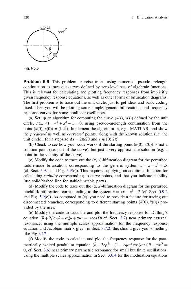
Fig. P5.5
320
5 Bifurcation Analysis
continuation to trace out curves defined by zero-level sets of algebraic functions.
This is relevant for calculating and plotting frequency responses from implicitly
given frequency response equations, as well as other forms of bifurcation diagrams.
The first problem is to trace out the unit circle, just to get ideas and basic coding
fixed. Then you will be plotting some simple, generic bifurcations, and frequency
response curves for some nonlinear oscillators.
(a) Set up an algorithm for computing the curve (a(s), x(s)) defined by the unit
circle, F(x, a) = a
2 + x
2
– 1 = 0, using pseudo-arclength continuation from the
point (a(0), x(0)) = ð
1
2 ;
ffiffi
3
p
2 Þ: Implement the algorithm in, e.g., MATLAB, and show
the predicted as well as corrected points, along with the known solution (i.e. the
unit circle), for a stepsize Ds = 2p/20 and s 2 [0; 2p].
(b) Check to see how your code works if the starting point (a(0), x(0)) is not a
solution point (i.e. part of the curve), but just a very approximate solution (e.g. a
point in the vicinity of the curve).
(c) Modify the code to trace out the (a, x)-bifurcation diagram for the perturbed
saddle-node bifurcation, corresponding to the generic system _
x ¼ a À x
2
þ 2x
(cf. Sect. 5.9.1 and Fig. 5.9(c)). This requires supplying an additional function for
calculating stability corresponding to curve points, and that you indicate stability
(use solid/dashed line for stable/unstable parts).
(d) Modify the code to trace out the (a, x)-bifurcation diagram for the perturbed
pitchfork bifurcation, corresponding to the system _
x ¼ ax À x
3
þ 2 (cf. Sect. 5.9.2
and Fig. 5.9(c)). As compared to (c), you need to provide a feature for tracing out
disconnected branches, corresponding to different starting points ð~ að0Þ; ~ xð0ÞÞ provided by the user.
(e) Modify the code to calculate and plot the frequency response for Duffing’s
equation ð€ u þ 2bx 0 _
u þ x
2
0 u þ cu
3
¼ q cos Xt;cf. Sect. 3.7) near primary external
resonance, using the multiple scales approximation for the frequency response
equation and Jacobian matrix given in Sect. 3.7.2; this should give you something
like Fig 3.17.
(f) Modify the code to calculate and plot the frequency response for the parametrically excited pendulum equation ð € h þ 2eb _
h þ 1 À eqx
2 cosðxsÞ
ð
Þ h þ ech
3
¼
0; cf. Sect. 3.6) near primary parametric resonance for small but finite oscillations,
using the multiple scales approximation in Sect. 3.6.4 for the modulation equations
Fig. P5.5
320
5 Bifurcation Analysis