

_
x ¼ l À x
2
þ ex:
ð5:32Þ
The perturbation ex is chosen instead of e, which would just add to l and
translate the bifurcation value. When l ! −e
2 /4 the perturbed system has a pair of
singular points at x =
1
2 (e ± (e
2 + 4l)
1/2
), but no singular points when l < −e
2 /4.
The Jacobian eigenvalues for the singular points are k = ±(e
2 + 4l)
1/2 . One
eigenvalue has a zero real part when l = –e
2 /4, which is thus a bifurcation value.
The corresponding bifurcation point is (l, x) = (−e
2 /4, e/2).
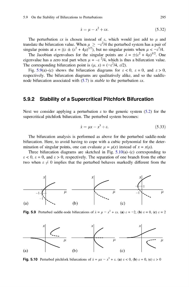
Fig. 5.9(a)–(c) shows the bifurcation diagrams for e < 0, e = 0, and e > 0,
respectively. The bifurcation diagrams are qualitatively alike, and so the saddlenode bifurcation associated with (5.7) is stable to the perturbation ex.
5.9.2 Stability of a Supercritical Pitchfork Bifurcation
Next we consider applying a perturbation e to the generic system (5.2) for the
supercritical pitchfork bifurcation. The perturbed system becomes:
_
x ¼ lx À x
3
þ e:
ð5:33Þ
The bifurcation analysis is performed as above for the perturbed saddle-node
bifurcation. Here, to avoid having to cope with a cubic polynomial for the determination of singular points, one can evaluate l = l(x) instead of x = x(l).
Three bifurcation diagrams are sketched in Fig. 5.10(a)–(c) corresponding to
e < 0, e = 0, and e > 0, respectively. The separation of one branch from the other
two when e 6 ¼ 0 implies that the perturbed behaves markedly different from the
Fig. 5.9 Perturbed saddle-node bifurcations of _
x = l − x
2 + ex. (a) e = −2, (b) e = 0, (c) e = 2
Fig. 5.10 Perturbed pitchfork bifurcations of _
x = lx − x
3 + e. (a) e < 0, (b) e = 0, (c) e > 0
5.9 On the Stability of Bifurcations to Perturbations
295
x ¼ l À x
2
þ ex:
ð5:32Þ
The perturbation ex is chosen instead of e, which would just add to l and
translate the bifurcation value. When l ! −e
2 /4 the perturbed system has a pair of
singular points at x =
1
2 (e ± (e
2 + 4l)
1/2
), but no singular points when l < −e
2 /4.
The Jacobian eigenvalues for the singular points are k = ±(e
2 + 4l)
1/2 . One
eigenvalue has a zero real part when l = –e
2 /4, which is thus a bifurcation value.
The corresponding bifurcation point is (l, x) = (−e
2 /4, e/2).
Fig. 5.9(a)–(c) shows the bifurcation diagrams for e < 0, e = 0, and e > 0,
respectively. The bifurcation diagrams are qualitatively alike, and so the saddlenode bifurcation associated with (5.7) is stable to the perturbation ex.
5.9.2 Stability of a Supercritical Pitchfork Bifurcation
Next we consider applying a perturbation e to the generic system (5.2) for the
supercritical pitchfork bifurcation. The perturbed system becomes:
_
x ¼ lx À x
3
þ e:
ð5:33Þ
The bifurcation analysis is performed as above for the perturbed saddle-node
bifurcation. Here, to avoid having to cope with a cubic polynomial for the determination of singular points, one can evaluate l = l(x) instead of x = x(l).
Three bifurcation diagrams are sketched in Fig. 5.10(a)–(c) corresponding to
e < 0, e = 0, and e > 0, respectively. The separation of one branch from the other
two when e 6 ¼ 0 implies that the perturbed behaves markedly different from the
Fig. 5.9 Perturbed saddle-node bifurcations of _
x = l − x
2 + ex. (a) e = −2, (b) e = 0, (c) e = 2
Fig. 5.10 Perturbed pitchfork bifurcations of _
x = lx − x
3 + e. (a) e < 0, (b) e = 0, (c) e > 0
5.9 On the Stability of Bifurcations to Perturbations
295