

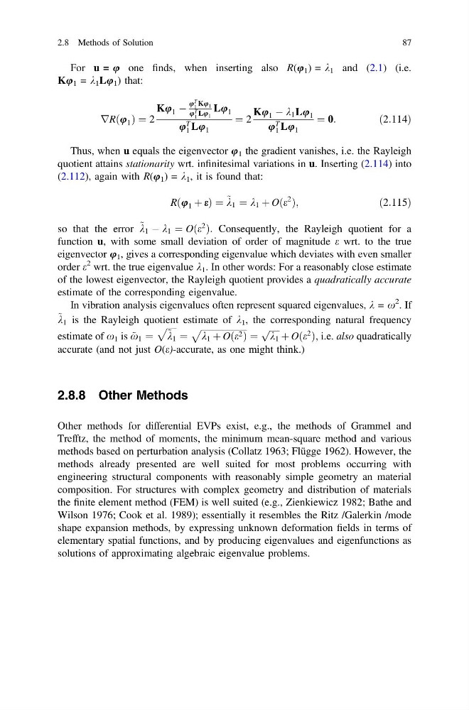
For u = u one finds, when inserting also R(u 1 ) = k 1 and (2.1) (i.e.
Ku 1 = k 1 Lu 1 ) that:
rRðu 1 Þ ¼ 2
Ku 1 À
u
T
1 Ku 1
u T
1
Lu 1
Lu 1
u T
1 Lu 1
¼ 2
Ku 1 À k 1 Lu 1
u T
1 Lu 1
¼ 0:
ð2:114Þ
Thus, when u equals the eigenvector u 1 the gradient vanishes, i.e. the Rayleigh
quotient attains stationarity wrt. infinitesimal variations in u. Inserting (2.114) into
(2.112), again with R(u 1 ) = k 1 , it is found that:
Rðu 1 þ eÞ ¼ ~ k 1 ¼ k 1 þ Oðe
2
Þ;
ð2:115Þ
so that the error ~ k 1 À k 1 ¼ Oðe
2
Þ: Consequently, the Rayleigh quotient for a
function u, with some small deviation of order of magnitude e wrt. to the true
eigenvector u 1 , gives a corresponding eigenvalue which deviates with even smaller
order e
2 wrt. the true eigenvalue k 1 . In other words: For a reasonably close estimate
of the lowest eigenvector, the Rayleigh quotient provides a quadratically accurate
estimate of the corresponding eigenvalue.
In vibration analysis eigenvalues often represent squared eigenvalues, k = x
2
. If
~ k 1 is the Rayleigh quotient estimate of k 1 , the corresponding natural frequency
estimate of x 1 is ~
x 1 ¼
ffiffiffiffi ffi
~ k 1
p
¼
ffiffiffiffiffiffiffiffiffiffiffiffiffiffiffiffiffiffiffiffiffi
k 1 þ Oðe 2 Þ
p
¼
ffiffiffiffi ffi
k 1
p þ Oðe
2
Þ; i.e. also quadratically
accurate (and not just O(e)-accurate, as one might think.)
2.8.8 Other Methods
Other methods for differential EVPs exist, e.g., the methods of Grammel and
Trefftz, the method of moments, the minimum mean-square method and various
methods based on perturbation analysis (Collatz 1963; Flügge 1962). However, the
methods already presented are well suited for most problems occurring with
engineering structural components with reasonably simple geometry an material
composition. For structures with complex geometry and distribution of materials
the finite element method (FEM) is well suited (e.g., Zienkiewicz 1982; Bathe and
Wilson 1976; Cook et al. 1989); essentially it resembles the Ritz /Galerkin /mode
shape expansion methods, by expressing unknown deformation fields in terms of
elementary spatial functions, and by producing eigenvalues and eigenfunctions as
solutions of approximating algebraic eigenvalue problems.
2.8 Methods of Solution
87
Ku 1 = k 1 Lu 1 ) that:
rRðu 1 Þ ¼ 2
Ku 1 À
u
T
1 Ku 1
u T
1
Lu 1
Lu 1
u T
1 Lu 1
¼ 2
Ku 1 À k 1 Lu 1
u T
1 Lu 1
¼ 0:
ð2:114Þ
Thus, when u equals the eigenvector u 1 the gradient vanishes, i.e. the Rayleigh
quotient attains stationarity wrt. infinitesimal variations in u. Inserting (2.114) into
(2.112), again with R(u 1 ) = k 1 , it is found that:
Rðu 1 þ eÞ ¼ ~ k 1 ¼ k 1 þ Oðe
2
Þ;
ð2:115Þ
so that the error ~ k 1 À k 1 ¼ Oðe
2
Þ: Consequently, the Rayleigh quotient for a
function u, with some small deviation of order of magnitude e wrt. to the true
eigenvector u 1 , gives a corresponding eigenvalue which deviates with even smaller
order e
2 wrt. the true eigenvalue k 1 . In other words: For a reasonably close estimate
of the lowest eigenvector, the Rayleigh quotient provides a quadratically accurate
estimate of the corresponding eigenvalue.
In vibration analysis eigenvalues often represent squared eigenvalues, k = x
2
. If
~ k 1 is the Rayleigh quotient estimate of k 1 , the corresponding natural frequency
estimate of x 1 is ~
x 1 ¼
ffiffiffiffi ffi
~ k 1
p
¼
ffiffiffiffiffiffiffiffiffiffiffiffiffiffiffiffiffiffiffiffiffi
k 1 þ Oðe 2 Þ
p
¼
ffiffiffiffi ffi
k 1
p þ Oðe
2
Þ; i.e. also quadratically
accurate (and not just O(e)-accurate, as one might think.)
2.8.8 Other Methods
Other methods for differential EVPs exist, e.g., the methods of Grammel and
Trefftz, the method of moments, the minimum mean-square method and various
methods based on perturbation analysis (Collatz 1963; Flügge 1962). However, the
methods already presented are well suited for most problems occurring with
engineering structural components with reasonably simple geometry an material
composition. For structures with complex geometry and distribution of materials
the finite element method (FEM) is well suited (e.g., Zienkiewicz 1982; Bathe and
Wilson 1976; Cook et al. 1989); essentially it resembles the Ritz /Galerkin /mode
shape expansion methods, by expressing unknown deformation fields in terms of
elementary spatial functions, and by producing eigenvalues and eigenfunctions as
solutions of approximating algebraic eigenvalue problems.
2.8 Methods of Solution
87