

4.4 Constitutive Relations for Macro-fiber Composites
65
P
P
Θ
3
Θ
2
˜
Θ 3
˜
Θ 1
Θ
1
Fiber
hE
Fib er
˘
Θ 2
˘
Θ 1
Epoxy
PZT
Electrodes
˜
Θ 2
(a) MFC-d31 structure
Θ
3
Θ
2
˜
Θ 3
Θ
1
P
˜
Θ 1
+
+
+
+
+
-
-
Fiber
P
˜
Θ 2
hE
˘
Θ 2
˘
Θ 1
Fi be r, P
Epoxy
PZT
Electrodes
(b) MFC-d33 structure
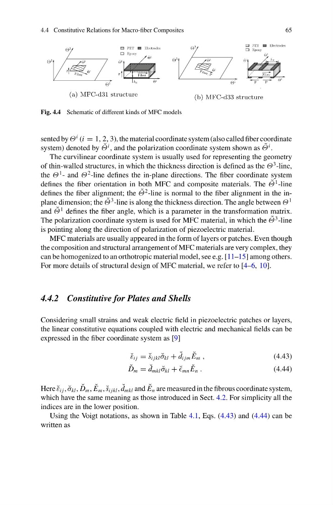
Fig. 4.4 Schematic of different kinds of MFC models
sented by Θ
i (i = 1, 2, 3), the material coordinate system (also called fiber coordinate
system) denoted by ˘
Θ
i , and the polarization coordinate system shown as ˜
Θ
i .
The curvilinear coordinate system is usually used for representing the geometry
of thin-walled structures, in which the thickness direction is defined as the Θ
3 -line,
the Θ
1 - and Θ
2 -line defines the in-plane directions. The fiber coordinate system
defines the fiber orientation in both MFC and composite materials. The ˘
Θ
1 -line
defines the fiber alignment; the ˘
Θ
2 -line is normal to the fiber alignment in the inplane dimension; the ˘
Θ
3 -line is along the thickness direction. The angle between Θ
1
and ˘
Θ
1 defines the fiber angle, which is a parameter in the transformation matrix.
The polarization coordinate system is used for MFC material, in which the ˜
Θ
3 -line
is pointing along the direction of polarization of piezoelectric material.
MFC materials are usually appeared in the form of layers or patches. Even though
the composition and structural arrangement of MFC materials are very complex, they
can be homogenized to an orthotropic material model, see e.g. [11–15] among others.
For more details of structural design of MFC material, we refer to [4–6, 10].
4.4.2 Constitutive for Plates and Shells
Considering small strains and weak electric field in piezoelectric patches or layers,
the linear constitutive equations coupled with electric and mechanical fields can be
expressed in the fiber coordinate system as [9]
˘
ε i j = ˘
s i jkl ˘
σ kl + ˘
d i jm ˘
E m ,
(4.43)
˘
D m = ˘
d mkl ˘
σ kl + ˘
mn ˘
E n .
(4.44)
Here ˘
ε i j , ˘
σ kl , ˘
D m , ˘
E m , ˘
s i jkl , ˘
d mkl and ˘
E n are measured in the fibrous coordinate system,
which have the same meaning as those introduced in Sect. 4.2. For simplicity all the
indices are in the lower position.
Using the Voigt notations, as shown in Table 4.1, Eqs. (4.43) and (4.44) can be
written as
65
P
P
Θ
3
Θ
2
˜
Θ 3
˜
Θ 1
Θ
1
Fiber
hE
Fib er
˘
Θ 2
˘
Θ 1
Epoxy
PZT
Electrodes
˜
Θ 2
(a) MFC-d31 structure
Θ
3
Θ
2
˜
Θ 3
Θ
1
P
˜
Θ 1
+
+
+
+
+
-
-
Fiber
P
˜
Θ 2
hE
˘
Θ 2
˘
Θ 1
Fi be r, P
Epoxy
PZT
Electrodes
(b) MFC-d33 structure
Fig. 4.4 Schematic of different kinds of MFC models
sented by Θ
i (i = 1, 2, 3), the material coordinate system (also called fiber coordinate
system) denoted by ˘
Θ
i , and the polarization coordinate system shown as ˜
Θ
i .
The curvilinear coordinate system is usually used for representing the geometry
of thin-walled structures, in which the thickness direction is defined as the Θ
3 -line,
the Θ
1 - and Θ
2 -line defines the in-plane directions. The fiber coordinate system
defines the fiber orientation in both MFC and composite materials. The ˘
Θ
1 -line
defines the fiber alignment; the ˘
Θ
2 -line is normal to the fiber alignment in the inplane dimension; the ˘
Θ
3 -line is along the thickness direction. The angle between Θ
1
and ˘
Θ
1 defines the fiber angle, which is a parameter in the transformation matrix.
The polarization coordinate system is used for MFC material, in which the ˜
Θ
3 -line
is pointing along the direction of polarization of piezoelectric material.
MFC materials are usually appeared in the form of layers or patches. Even though
the composition and structural arrangement of MFC materials are very complex, they
can be homogenized to an orthotropic material model, see e.g. [11–15] among others.
For more details of structural design of MFC material, we refer to [4–6, 10].
4.4.2 Constitutive for Plates and Shells
Considering small strains and weak electric field in piezoelectric patches or layers,
the linear constitutive equations coupled with electric and mechanical fields can be
expressed in the fiber coordinate system as [9]
˘
ε i j = ˘
s i jkl ˘
σ kl + ˘
d i jm ˘
E m ,
(4.43)
˘
D m = ˘
d mkl ˘
σ kl + ˘
mn ˘
E n .
(4.44)
Here ˘
ε i j , ˘
σ kl , ˘
D m , ˘
E m , ˘
s i jkl , ˘
d mkl and ˘
E n are measured in the fibrous coordinate system,
which have the same meaning as those introduced in Sect. 4.2. For simplicity all the
indices are in the lower position.
Using the Voigt notations, as shown in Table 4.1, Eqs. (4.43) and (4.44) can be
written as