

5.5 Total Lagrangian Formulation
87
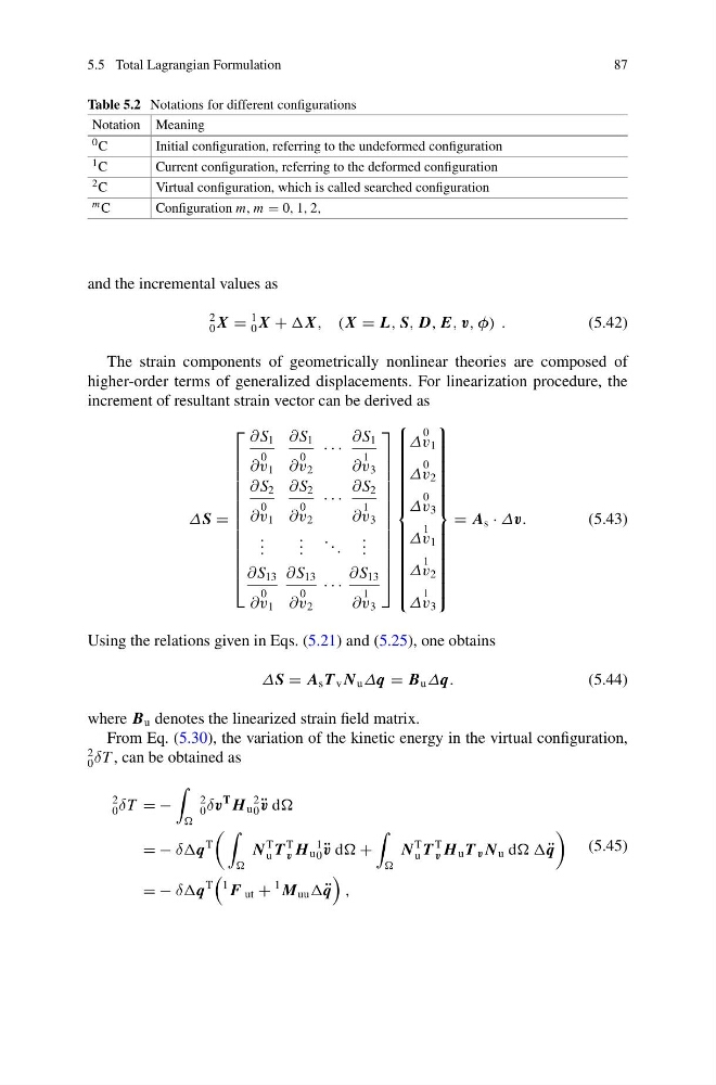
Table 5.2 Notations for different configurations
Notation Meaning
0 C
Initial configuration, referring to the undeformed configuration
1 C
Current configuration, referring to the deformed configuration
2 C
Virtual configuration, which is called searched configuration
m C
Configuration m, m = 0, 1, 2,
and the incremental values as
2
0 X =
1
0 X + X, (X = L, S, D, E, v, φ) .
(5.42)
The strain components of geometrically nonlinear theories are composed of
higher-order terms of generalized displacements. For linearization procedure, the
increment of resultant strain vector can be derived as
ΔS =
⎡
⎢
⎢
⎢
⎢
⎢
⎢
⎢
⎢
⎢
⎢
⎢
⎢
⎣
∂ S 1
∂
0
v 1
∂ S 1
∂
0
v 2
· · ·
∂ S 1
∂
1
v 3
∂ S 2
∂
0
v 1
∂ S 2
∂
0
v 2
· · ·
∂ S 2
∂
1
v 3
. . .
. . .
. . .
. . .
∂ S 13
∂
0
v 1
∂ S 13
∂
0
v 2
· · ·
∂ S 13
∂
1
v 3
⎤
⎥
⎥
⎥
⎥
⎥
⎥
⎥
⎥
⎥
⎥
⎥
⎥
⎦
⎧
⎪ ⎪ ⎪ ⎪ ⎪ ⎪ ⎪ ⎪ ⎪ ⎪ ⎪ ⎪ ⎪ ⎨
⎪ ⎪ ⎪ ⎪ ⎪ ⎪ ⎪ ⎪ ⎪ ⎪ ⎪ ⎪ ⎪ ⎩
Δ
0
v 1
Δ
0
v 2
Δ
0
v 3
Δ
1
v 1
Δ
1
v 2
Δ
1
v 3
⎫
⎪ ⎪ ⎪ ⎪ ⎪ ⎪ ⎪ ⎪ ⎪ ⎪ ⎪ ⎪ ⎪ ⎬
⎪ ⎪ ⎪ ⎪ ⎪ ⎪ ⎪ ⎪ ⎪ ⎪ ⎪ ⎪ ⎪ ⎭
= A s · Δv.
(5.43)
Using the relations given in Eqs. (5.21) and (5.25), one obtains
ΔS = A s T v N u Δq = B u Δq.
(5.44)
where B u denotes the linearized strain field matrix.
From Eq. (5.30), the variation of the kinetic energy in the virtual configuration,
2
0 δT , can be obtained as
2
0 δT = −
2
0 δv
T H u
2
0 ¨
v d
= − δq
T
N
T
u T
T
v H u
1
0 ¨
v d +
N
T
u T
T
v H u T v N u d ¨
q
= − δq
T
1 F ut +
1 M uu ¨
q
,
(5.45)
87
Table 5.2 Notations for different configurations
Notation Meaning
0 C
Initial configuration, referring to the undeformed configuration
1 C
Current configuration, referring to the deformed configuration
2 C
Virtual configuration, which is called searched configuration
m C
Configuration m, m = 0, 1, 2,
and the incremental values as
2
0 X =
1
0 X + X, (X = L, S, D, E, v, φ) .
(5.42)
The strain components of geometrically nonlinear theories are composed of
higher-order terms of generalized displacements. For linearization procedure, the
increment of resultant strain vector can be derived as
ΔS =
⎡
⎢
⎢
⎢
⎢
⎢
⎢
⎢
⎢
⎢
⎢
⎢
⎢
⎣
∂ S 1
∂
0
v 1
∂ S 1
∂
0
v 2
· · ·
∂ S 1
∂
1
v 3
∂ S 2
∂
0
v 1
∂ S 2
∂
0
v 2
· · ·
∂ S 2
∂
1
v 3
. . .
. . .
. . .
. . .
∂ S 13
∂
0
v 1
∂ S 13
∂
0
v 2
· · ·
∂ S 13
∂
1
v 3
⎤
⎥
⎥
⎥
⎥
⎥
⎥
⎥
⎥
⎥
⎥
⎥
⎥
⎦
⎧
⎪ ⎪ ⎪ ⎪ ⎪ ⎪ ⎪ ⎪ ⎪ ⎪ ⎪ ⎪ ⎪ ⎨
⎪ ⎪ ⎪ ⎪ ⎪ ⎪ ⎪ ⎪ ⎪ ⎪ ⎪ ⎪ ⎪ ⎩
Δ
0
v 1
Δ
0
v 2
Δ
0
v 3
Δ
1
v 1
Δ
1
v 2
Δ
1
v 3
⎫
⎪ ⎪ ⎪ ⎪ ⎪ ⎪ ⎪ ⎪ ⎪ ⎪ ⎪ ⎪ ⎪ ⎬
⎪ ⎪ ⎪ ⎪ ⎪ ⎪ ⎪ ⎪ ⎪ ⎪ ⎪ ⎪ ⎪ ⎭
= A s · Δv.
(5.43)
Using the relations given in Eqs. (5.21) and (5.25), one obtains
ΔS = A s T v N u Δq = B u Δq.
(5.44)
where B u denotes the linearized strain field matrix.
From Eq. (5.30), the variation of the kinetic energy in the virtual configuration,
2
0 δT , can be obtained as
2
0 δT = −
2
0 δv
T H u
2
0 ¨
v d
= − δq
T
N
T
u T
T
v H u
1
0 ¨
v d +
N
T
u T
T
v H u T v N u d ¨
q
= − δq
T
1 F ut +
1 M uu ¨
q
,
(5.45)