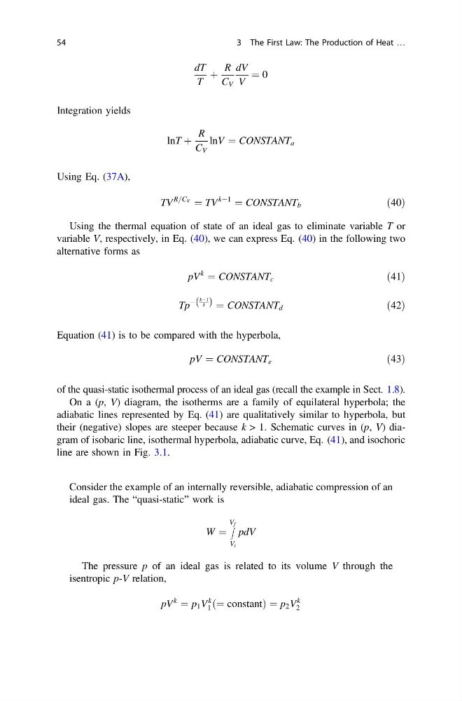
dT
T
þ
R
C V
dV
V
¼ 0
Integration yields
lnT þ
R
C V
lnV ¼ CONSTANT a
Using Eq. (37A),
TV
R=C V ¼ TV
kÀ1
¼ CONSTANT b
ð40Þ
Using the thermal equation of state of an ideal gas to eliminate variable T or
variable V, respectively, in Eq. (40), we can express Eq. (40) in the following two
alternative forms as
pV
k
¼ CONSTANT c
ð41Þ
Tp
À
kÀ1
k
ð Þ ¼ CONSTANT d
ð42Þ
Equation (41) is to be compared with the hyperbola,
pV ¼ CONSTANT e
ð43Þ
of the quasi-static isothermal process of an ideal gas (recall the example in Sect. 1.8).
On a (p, V) diagram, the isotherms are a family of equilateral hyperbola; the
adiabatic lines represented by Eq. (41) are qualitatively similar to hyperbola, but
their (negative) slopes are steeper because k > 1. Schematic curves in (p, V) diagram of isobaric line, isothermal hyperbola, adiabatic curve, Eq. (41), and isochoric
line are shown in Fig. 3.1.
Consider the example of an internally reversible, adiabatic compression of an
ideal gas. The “quasi-static” work is
W ¼
Z
V f
V i
pdV
The pressure p of an ideal gas is related to its volume V through the
isentropic p-V relation,
pV
k
¼ p 1 V
k
1 ð¼ constantÞ ¼ p 2 V
k
2
54
3 The First Law: The Production of Heat …