

68
3 Continuum Mechanics and Nonlinear Elasticity
of the bar changes from L to . Since the cells in a tissue likely respond to the local
mechanical environment, it is important to know how the deformation changes with
position along the bar.
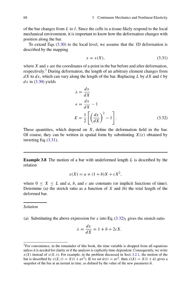
To extend Eqs. (3.30) to the local level, we assume that the 1D deformation is
described by the mapping
x = x(X),
(3.31)
where X and x are the coordinates of a point in the bar before and after deformation,
respectively. 3 During deformation, the length of an arbitrary element changes from
dX to dx, which can vary along the length of the bar. Replacing L by dX and by
dx in (3.30) yields
λ =
dx
dX
=
dx
dX
− 1
E =
1
2
dx
dX
2
− 1
.
(3.32)
These quantities, which depend on X, define the deformation field in the bar.
Of course, they can be written in spatial form by substituting X(x) obtained by
inverting Eq. (3.31).
Example 3.8 The motion of a bar with undeformed length L is described by the
relation
x(X) = a + (1 + b)X + cX
2 ,
where 0 ≤ X ≤ L and a, b, and c are constants (or implicit functions of time).
Determine (a) the stretch ratio as a function of X and (b) the total length of the
deformed bar.
Solution
(a) Substituting the above expression for x into Eq. (3.32) 1 gives the stretch ratio
λ =
dx
dX
= 1 + b + 2cX.
3 For convenience, in the remainder of this book, the time variable is dropped from all equations
unless it is needed for clarity or if the analysis is explicitly time-dependent. Consequently, we write
x(X) instead of x(X, t). For example, in the problem discussed in Sect. 3.2.1, the motion of the
bar is described by x(X, t) = X(1 + αt 2 ). If we set ¯
α(t) = αt 2 , then x(X) = X(1 + ¯
α) gives a
snapshot of the bar at an instant in time, as defined by the value of the new parameter ¯
α.
3 Continuum Mechanics and Nonlinear Elasticity
of the bar changes from L to . Since the cells in a tissue likely respond to the local
mechanical environment, it is important to know how the deformation changes with
position along the bar.
To extend Eqs. (3.30) to the local level, we assume that the 1D deformation is
described by the mapping
x = x(X),
(3.31)
where X and x are the coordinates of a point in the bar before and after deformation,
respectively. 3 During deformation, the length of an arbitrary element changes from
dX to dx, which can vary along the length of the bar. Replacing L by dX and by
dx in (3.30) yields
λ =
dx
dX
=
dx
dX
− 1
E =
1
2
dx
dX
2
− 1
.
(3.32)
These quantities, which depend on X, define the deformation field in the bar.
Of course, they can be written in spatial form by substituting X(x) obtained by
inverting Eq. (3.31).
Example 3.8 The motion of a bar with undeformed length L is described by the
relation
x(X) = a + (1 + b)X + cX
2 ,
where 0 ≤ X ≤ L and a, b, and c are constants (or implicit functions of time).
Determine (a) the stretch ratio as a function of X and (b) the total length of the
deformed bar.
Solution
(a) Substituting the above expression for x into Eq. (3.32) 1 gives the stretch ratio
λ =
dx
dX
= 1 + b + 2cX.
3 For convenience, in the remainder of this book, the time variable is dropped from all equations
unless it is needed for clarity or if the analysis is explicitly time-dependent. Consequently, we write
x(X) instead of x(X, t). For example, in the problem discussed in Sect. 3.2.1, the motion of the
bar is described by x(X, t) = X(1 + αt 2 ). If we set ¯
α(t) = αt 2 , then x(X) = X(1 + ¯
α) gives a
snapshot of the bar at an instant in time, as defined by the value of the new parameter ¯
α.