

422
8 Morphogenesis
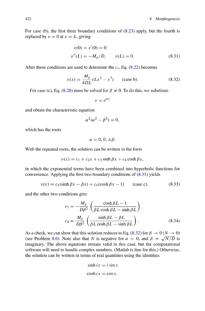
For case (b), the first three boundary conditions of (8.23) apply, but the fourth is
replaced by v = 0 at x = L, giving
v(0) = v
(0) = 0
v
(L) = −M g /D,
v(L) = 0.
(8.31)
After these conditions are used to determine the c i , Eq. (8.22) becomes
v(x) =
M g
4DL
(Lx
2
− x
3 )
(case b).
(8.32)
For case (c), Eq. (8.28) must be solved for β = 0. To do this, we substitute
v = e
αx
and obtain the characteristic equation
α
2 (α
2
− β
2 ) = 0,
which has the roots
α = 0, 0, ±β.
With the repeated roots, the solution can be written in the form
v(x) = c 1 + c 2 x + c 3 sinh βx + c 4 cosh βx,
in which the exponential terms have been combined into hyperbolic functions for
convenience. Applying the first two boundary conditions of (8.31) yields
v(x) = c 3 (sinh βx − βx) + c 4 (cosh βx − 1)
(case c),
(8.33)
and the other two conditions give
c 3 = −
M g
Dβ 2
cosh βL − 1
βL cosh βL − sinh βL
c 4 =
M g
Dβ 2
sinh βL − βL
βL cosh βL − sinh βL
.
(8.34)
As a check, we can show that this solution reduces to Eq. (8.32) for β → 0 (N → 0)
(see Problem 8.6). Note also that N is negative for a > 0, and β =
√
N/D is
imaginary. The above equations remain valid in this case, but the computational
software will need to handle complex numbers. (Matlab is fine for this.) Otherwise,
the solution can be written in terms of real quantities using the identities
sinh ix = i sin x
cosh ix = cos x.
8 Morphogenesis
For case (b), the first three boundary conditions of (8.23) apply, but the fourth is
replaced by v = 0 at x = L, giving
v(0) = v
(0) = 0
v
(L) = −M g /D,
v(L) = 0.
(8.31)
After these conditions are used to determine the c i , Eq. (8.22) becomes
v(x) =
M g
4DL
(Lx
2
− x
3 )
(case b).
(8.32)
For case (c), Eq. (8.28) must be solved for β = 0. To do this, we substitute
v = e
αx
and obtain the characteristic equation
α
2 (α
2
− β
2 ) = 0,
which has the roots
α = 0, 0, ±β.
With the repeated roots, the solution can be written in the form
v(x) = c 1 + c 2 x + c 3 sinh βx + c 4 cosh βx,
in which the exponential terms have been combined into hyperbolic functions for
convenience. Applying the first two boundary conditions of (8.31) yields
v(x) = c 3 (sinh βx − βx) + c 4 (cosh βx − 1)
(case c),
(8.33)
and the other two conditions give
c 3 = −
M g
Dβ 2
cosh βL − 1
βL cosh βL − sinh βL
c 4 =
M g
Dβ 2
sinh βL − βL
βL cosh βL − sinh βL
.
(8.34)
As a check, we can show that this solution reduces to Eq. (8.32) for β → 0 (N → 0)
(see Problem 8.6). Note also that N is negative for a > 0, and β =
√
N/D is
imaginary. The above equations remain valid in this case, but the computational
software will need to handle complex numbers. (Matlab is fine for this.) Otherwise,
the solution can be written in terms of real quantities using the identities
sinh ix = i sin x
cosh ix = cos x.