

390
7 Remodeling
It is important to note the following. As shown in earlier problems, the state of
strain in a homogeneous, incompressible membrane is completely determined by
prescribed edge displacements. And since k n − depends on strain, the present model
is based purely on kinematics. Thus, a solution can be obtained without the need to
consider stress and material properties. This would not be possible if k n − depends
on stress, as in Eq. (7.69).
7.8.3 Solution Procedure
In the reference state at t = 0, the volume fractions φ n
0 = J n
0 = 1/N (
N
n=1 φ n
0 =
1) are the same for all fiber families. Given λ x (t) and λ y (t), we step in time and
compute λ n , λ n∗ , k n − , and q n using Eqs. (7.105), (7.106), (7.101), and (7.108),
respectively, at each time step.
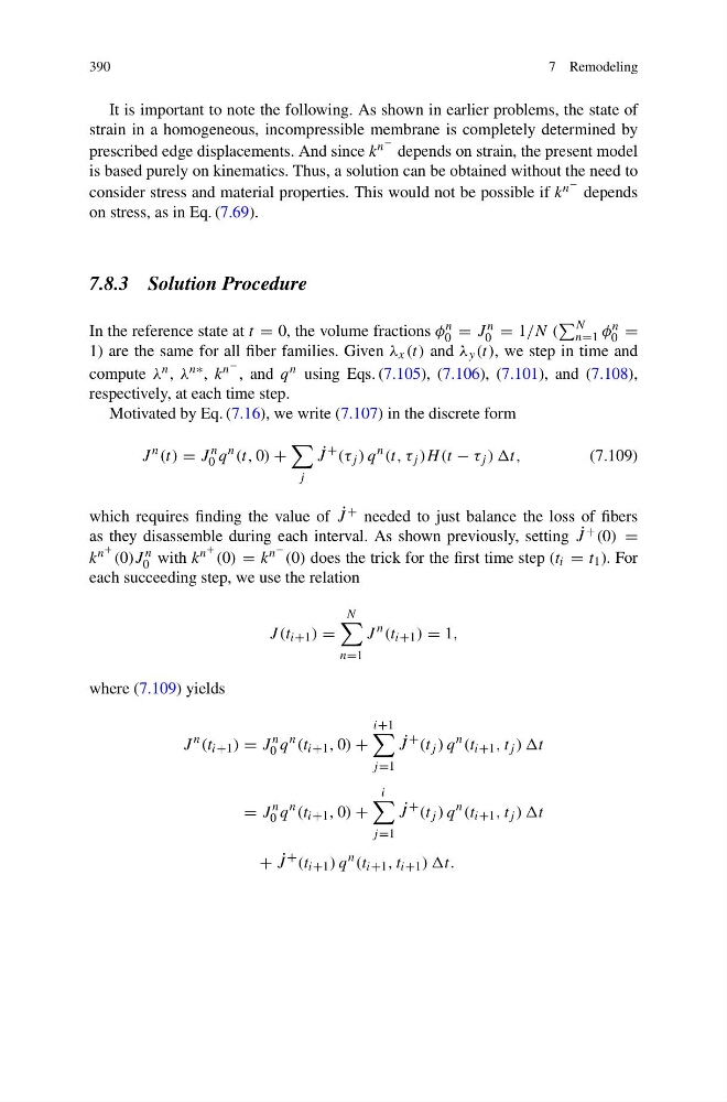
Motivated by Eq. (7.16), we write (7.107) in the discrete form
J
n (t) = J
n
0 q
n (t, 0) +
j
˙
J
+ (τ j ) q
n (t, τ j )H (t − τ j ) )t,
(7.109)
which requires finding the value of ˙
J + needed to just balance the loss of fibers
as they disassemble during each interval. As shown previously, setting ˙
J + (0) =
k n + (0)J n
0 with k n + (0) = k n − (0) does the trick for the first time step (t i = t 1 ). For
each succeeding step, we use the relation
J (t i+1 ) =
N
n=1
J
n (t i+1 ) = 1,
where (7.109) yields
J
n (t i+1 ) = J
n
0 q
n (t i+1 , 0) +
i+1
j =1
˙
J
+ (t j ) q
n (t i+1 , t j ) )t
= J
n
0 q
n (t i+1 , 0) +
i
j =1
˙
J
+ (t j ) q
n (t i+1 , t j ) )t
+ ˙
J
+ (t i+1 ) q
n (t i+1 , t i+1 ) )t.
7 Remodeling
It is important to note the following. As shown in earlier problems, the state of
strain in a homogeneous, incompressible membrane is completely determined by
prescribed edge displacements. And since k n − depends on strain, the present model
is based purely on kinematics. Thus, a solution can be obtained without the need to
consider stress and material properties. This would not be possible if k n − depends
on stress, as in Eq. (7.69).
7.8.3 Solution Procedure
In the reference state at t = 0, the volume fractions φ n
0 = J n
0 = 1/N (
N
n=1 φ n
0 =
1) are the same for all fiber families. Given λ x (t) and λ y (t), we step in time and
compute λ n , λ n∗ , k n − , and q n using Eqs. (7.105), (7.106), (7.101), and (7.108),
respectively, at each time step.
Motivated by Eq. (7.16), we write (7.107) in the discrete form
J
n (t) = J
n
0 q
n (t, 0) +
j
˙
J
+ (τ j ) q
n (t, τ j )H (t − τ j ) )t,
(7.109)
which requires finding the value of ˙
J + needed to just balance the loss of fibers
as they disassemble during each interval. As shown previously, setting ˙
J + (0) =
k n + (0)J n
0 with k n + (0) = k n − (0) does the trick for the first time step (t i = t 1 ). For
each succeeding step, we use the relation
J (t i+1 ) =
N
n=1
J
n (t i+1 ) = 1,
where (7.109) yields
J
n (t i+1 ) = J
n
0 q
n (t i+1 , 0) +
i+1
j =1
˙
J
+ (t j ) q
n (t i+1 , t j ) )t
= J
n
0 q
n (t i+1 , 0) +
i
j =1
˙
J
+ (t j ) q
n (t i+1 , t j ) )t
+ ˙
J
+ (t i+1 ) q
n (t i+1 , t i+1 ) )t.