

388
7 Remodeling
D
n
0
y
Initial state
Cyclic stretch
Remodeled state
)
c
(
)
b
(
)
a
(
x
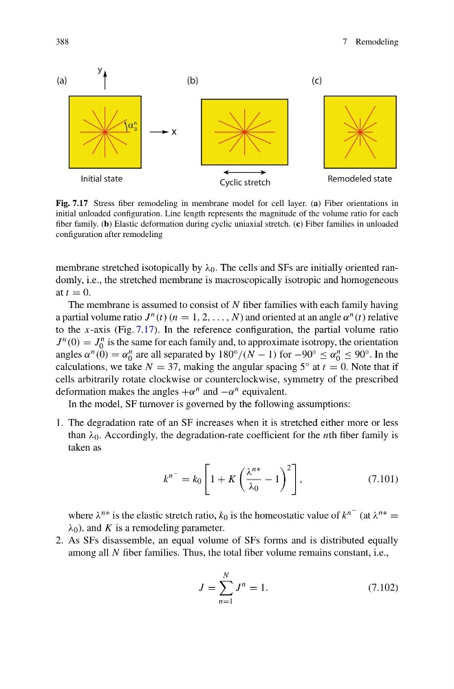
Fig. 7.17 Stress fiber remodeling in membrane model for cell layer. (a) Fiber orientations in
initial unloaded configuration. Line length represents the magnitude of the volume ratio for each
fiber family. (b) Elastic deformation during cyclic uniaxial stretch. (c) Fiber families in unloaded
configuration after remodeling
membrane stretched isotopically by λ 0 . The cells and SFs are initially oriented randomly, i.e., the stretched membrane is macroscopically isotropic and homogeneous
at t = 0.
The membrane is assumed to consist of N fiber families with each family having
a partial volume ratio J n (t) (n = 1, 2, . . . , N) and oriented at an angle α n (t) relative
to the x-axis (Fig. 7.17). In the reference configuration, the partial volume ratio
J n (0) = J n
0 is the same for each family and, to approximate isotropy, the orientation
angles α n (0) = α n
0 are all separated by 180 ◦ /(N − 1) for −90 ◦ ≤ α n
0 ≤ 90 ◦ . In the
calculations, we take N = 37, making the angular spacing 5 ◦ at t = 0. Note that if
cells arbitrarily rotate clockwise or counterclockwise, symmetry of the prescribed
deformation makes the angles +α n and −α n equivalent.
In the model, SF turnover is governed by the following assumptions:
1. The degradation rate of an SF increases when it is stretched either more or less
than λ 0 . Accordingly, the degradation-rate coefficient for the nth fiber family is
taken as
k
n − = k 0
1 + K
λ n∗
λ 0
− 1
2
,
(7.101)
where λ n∗ is the elastic stretch ratio, k 0 is the homeostatic value of k n − (at λ n∗ =
λ 0 ), and K is a remodeling parameter.
2. As SFs disassemble, an equal volume of SFs forms and is distributed equally
among all N fiber families. Thus, the total fiber volume remains constant, i.e.,
J =
N
n=1
J
n
= 1.
(7.102)
7 Remodeling
D
n
0
y
Initial state
Cyclic stretch
Remodeled state
)
c
(
)
b
(
)
a
(
x
Fig. 7.17 Stress fiber remodeling in membrane model for cell layer. (a) Fiber orientations in
initial unloaded configuration. Line length represents the magnitude of the volume ratio for each
fiber family. (b) Elastic deformation during cyclic uniaxial stretch. (c) Fiber families in unloaded
configuration after remodeling
membrane stretched isotopically by λ 0 . The cells and SFs are initially oriented randomly, i.e., the stretched membrane is macroscopically isotropic and homogeneous
at t = 0.
The membrane is assumed to consist of N fiber families with each family having
a partial volume ratio J n (t) (n = 1, 2, . . . , N) and oriented at an angle α n (t) relative
to the x-axis (Fig. 7.17). In the reference configuration, the partial volume ratio
J n (0) = J n
0 is the same for each family and, to approximate isotropy, the orientation
angles α n (0) = α n
0 are all separated by 180 ◦ /(N − 1) for −90 ◦ ≤ α n
0 ≤ 90 ◦ . In the
calculations, we take N = 37, making the angular spacing 5 ◦ at t = 0. Note that if
cells arbitrarily rotate clockwise or counterclockwise, symmetry of the prescribed
deformation makes the angles +α n and −α n equivalent.
In the model, SF turnover is governed by the following assumptions:
1. The degradation rate of an SF increases when it is stretched either more or less
than λ 0 . Accordingly, the degradation-rate coefficient for the nth fiber family is
taken as
k
n − = k 0
1 + K
λ n∗
λ 0
− 1
2
,
(7.101)
where λ n∗ is the elastic stretch ratio, k 0 is the homeostatic value of k n − (at λ n∗ =
λ 0 ), and K is a remodeling parameter.
2. As SFs disassemble, an equal volume of SFs forms and is distributed equally
among all N fiber families. Thus, the total fiber volume remains constant, i.e.,
J =
N
n=1
J
n
= 1.
(7.102)